Lavorare con le liste

R per utenti SAS

Melinda Higgins, PhD

Research Professor/Senior Biostatistician Emory University

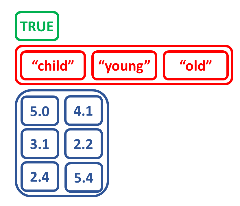
Crea una lista combinando altri oggetti

# Create logical scalar
logic_scalar <- TRUE
logic_scalar

[1] TRUE

elemento scalare TRUE

Crea una lista combinando altri oggetti

# Create character vector age_charvec
age_charvec <- c("child", "young", "old")
age_charvec

[1] "child" "young" "old"

scalare TRUE e vettore di caratteri

Crea una lista combinando altri oggetti

# Create matrix num_matrix
a <- c(5.0, 3.1, 2.4)
b <- c(4.1, 2.2, 5.4)
num_matrix <- matrix(c(a, b),
                     nrow = 3,
                     ncol = 2)
num_matrix

     [,1] [,2]
[1,]  5.0  4.1
[2,]  3.1  2.2
[3,]  2.4  5.4

scalare TRUE, vettore di caratteri e matrice

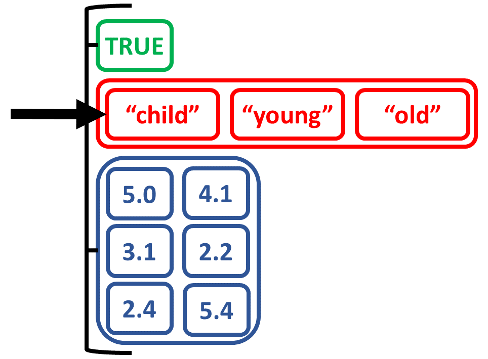
Crea una lista combinando oggetti di tipi diversi

# Create list from scalar, vector, matrix
list_logicagemtx <-
  list(logic_scalar, age_charvec, num_matrix)
list_logicagemtx

[[1]]
[1] TRUE

[[2]]
[1] "child" "young" "old"  

[[3]]
     [,1] [,2]
[1,]  5.0  4.1
[2,]  3.1  2.2
[3,]  2.4  5.4

tutti gli elementi combinati in una lista

Elementi della lista con nome

# Name the elements of the list, view names
names(list_logicagemtx) <- c("logicalValue", "ageDescription", "numericMatrix")
names(list_logicagemtx)

[1] "logicalValue"   "ageDescription" "numericMatrix"

# Get structure of list_logicagemtx
str(list_logicagemtx)

List of 3
 $ logicalValue  : logi TRUE
 $ ageDescription: chr [1:3] "child" "young" "old"
 $ numericMatrix : num [1:3, 1:2] 5 3.1 2.4 4.1 2.2 5.4

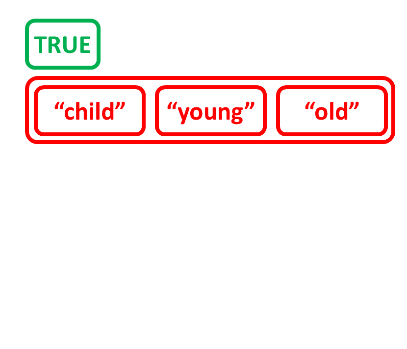
Seleziona elementi da una lista per nome

# Select ageDescription with $
list_logicagemtx$ageDescription

[1] "child" "young" "old"

# Check class of the ageDescription element
class(list_logicagemtx$ageDescription)

[1] "character"

# Confirm vector class
is.vector(list_logicagemtx$ageDescription)

[1] TRUE

seleziona un vettore di caratteri da una lista

Output di Hmisc

# Run Hmisc::describe() for sex and bmi
davisHmisc <- daviskeep %>%
  select(sex, bmi) %>%
  Hmisc::describe()

# Structure of Hmisc::describe() output
str(davisHmisc)

List of 2
 $ sex:List of 5
  ..$ descript: chr "sex"
  ..$ units   : NULL
  ..$ format  : NULL
  ..$ counts  : Named num [1:3] 199 0 2
  .. ..- attr(*, "names")= chr [1:3] "n" "missing" "distinct"
  ..$ values  :List of 2
  .. ..$ value    : chr [1:2] "F" "M"
  .. ..$ frequency: num [1:2(1d)] 111 88
  ..- attr(*, "class")= chr "describe"
 $ bmi:List of 6
  ..$ descript: chr "bmi"

... rest of output omitted ...

Output di Hmisc

# View sex element of Hmisc describe output
davisHmisc$sex

sex
       n  missing distinct
     199        0        2

Value          F     M
Frequency    111    88
Proportion 0.558 0.442

# Confirm the describe class is also a list
is.list(davisHmisc$sex)

[1] TRUE

Output di Hmisc

# View names of elements in davisHmisc$sex
names(davisHmisc$sex)

[1] "descript" "units" "format" "counts" "values"

# Use $ selector again to display counts for sex
davisHmisc$sex$counts

  n  missing distinct
199        0        2

Output dei test di correlazione

# Save output from psych::corr.test()
daviscorr <- daviskeep %>%
  select(bmi, weight, height) %>%
  psych::corr.test()

# View names of 11 elements in psych::corr output
names(daviscorr)

 [1]  "r"      "n"      "t"      "p"      "se"     
 [6]  "sef"    "adjust" "sym"    "ci"     "ci.adj"
 [11] "Call"

Output dei test di correlazione

daviscorr$p

                bmi       weight       height
bmi    0.000000e+00 2.569508e-64 3.628533e-08
weight 8.565028e-65 0.000000e+00 4.017148e-40
height 3.628533e-08 2.008574e-40 0.000000e+00

daviscorr$ci

                lower         r     upper            p
bmi-weght   0.8410885 0.8775201 0.9060257 8.565028e-65
bmi-heght   0.2524241 0.3782344 0.4914688 3.628533e-08
weght-heght 0.7074835 0.7707306 0.8217303 2.008574e-40

Output dei t-test

# UNPOOLED t-test bmi by sex
davisunpooled <- t.test(bmi ~ sex,
                        data = daviskeep)
class(davisunpooled)

[1] "htest"

is.list(davisunpooled)

[1] TRUE

names(davispooled)

[1] "statistic"   "parameter"   
[3] "p.value"     "conf.int"    
[5] "estimate"    "null.value"  
[7] "alternative" "method"      
[9] "data.name"

Output dei test chi-quadro

# Create table object of bmigt25 by sex and view table
tablebmisex <- daviskeep %>%
  with(table(bmigt25, sex))
daviscs <- chisq.test(tablebmisex)
class(daviscs)

[1] "htest"

names(daviscs)

[1] "statistic" "parameter" "p.value"   "method"    "data.name" "observed"
[7] "expected"  "residuals" "stdres"

Output della classe lista htest

Output t-test

davisunpooled$statistic
davisunpooled$parameter
davisunpooled$p.value

        t
-7.515792

      df
149.4533

[1] 4.818621e-12

Output test chi-quadro

daviscs$observed

                 sex
bmigt25             F   M
  1. underwt/norm 107  54
  2. overwt/obese   4  34

daviscs$expected

                 sex
bmigt25                  F        M
  1. underwt/norm 89.80402 71.19598
  2. overwt/obese 21.19598 16.80402

Lavoriamo con gli output delle liste per personalizzare i risultati dell’analisi delle abaloni.

R per utenti SAS