Imputazione con alberi
Gestione dei dati mancanti con imputazioni in R

Michal Oleszak
Machine Learning Engineer
Approccio di imputazione ad alberi
Usa modelli di machine learning per prevedere i valori mancanti!
- Approccio non parametrico: nessuna assunzione sulle relazioni tra variabili.
- Cattura pattern non lineari complessi.
- Spesso più accurato dei modelli statistici semplici.
In questo corso: pacchetto missForest, basato su randomForest
Alberi decisionali
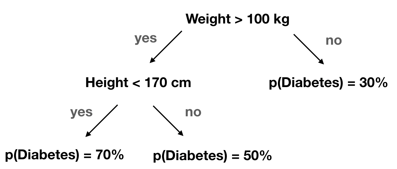
Random forest
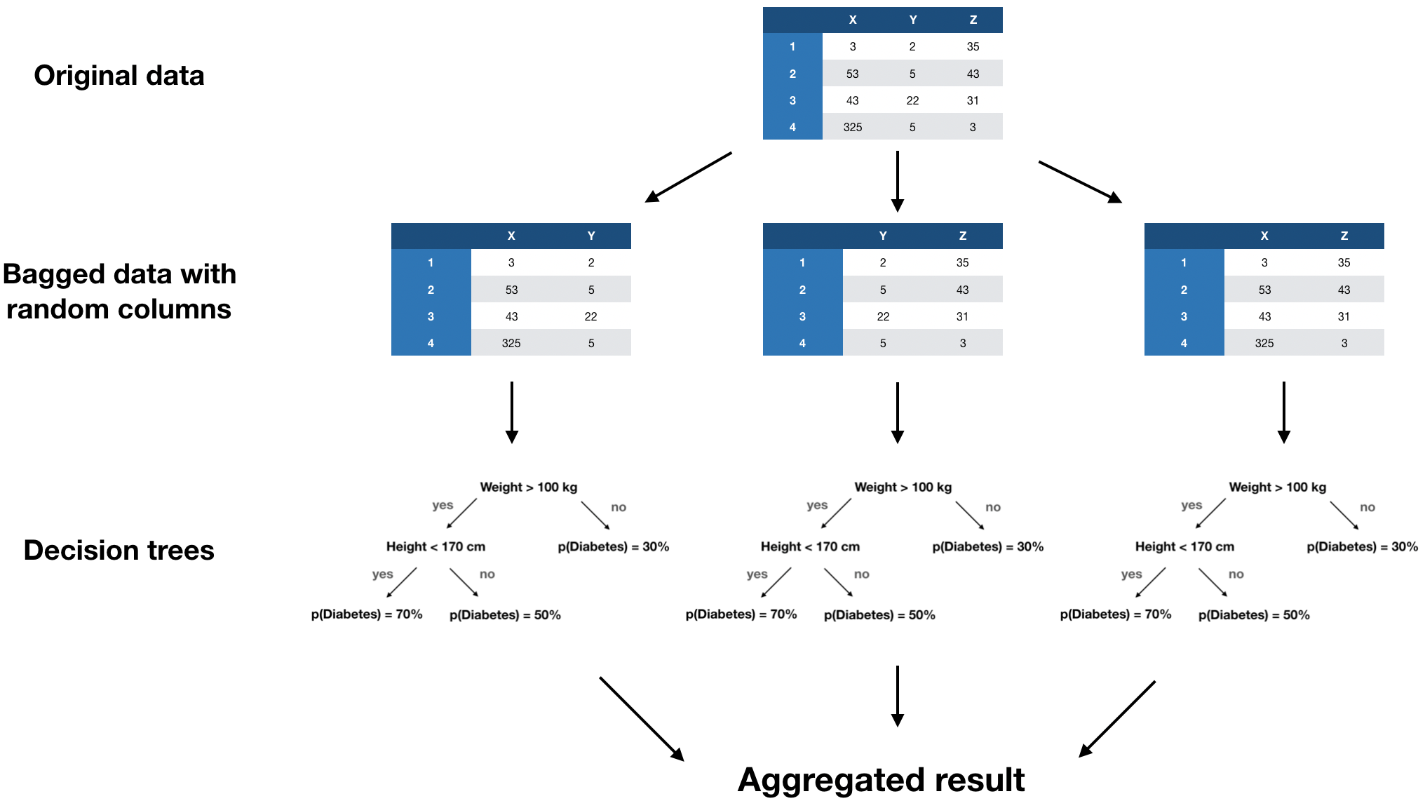
Algoritmo missForest
- Fai una stima iniziale dei mancanti con imputazione per media.
- Ordina le variabili in ordine crescente di valori mancanti.
- Per ogni variabile x:
- Allena una random forest sulla parte osservata di x (altre variabili come predittori).
- Usala per prevedere la parte mancante di x.
- Ripeti il punto 3 finché i valori imputati cambiano poco.
missForest in pratica
nhanes %>% is.na() %>% colSums()
Age     Gender     Weight     Height   Diabetes    TotChol      Pulse PhysActive
  0          0          9          8          1         85         32         26
library(missForest)
imp_res <- missForest(nhanes)
nhanes_imp  <- imp_res$ximp
nhanes_imp %>% is.na() %>% colSums()
Age     Gender     Weight     Height   Diabetes    TotChol      Pulse PhysActive
  0          0          0          0          0          0          0          0
Errore di imputazione
missForest() fornisce una stima OOB (out-of-bag) dell’errore di imputazione:
- NRMSE (errore quadratico medio normalizzato) per variabili continue.
- PFC (quota di classificazioni errate) per variabili categoriche.
In entrambi i casi, buone prestazioni → valore vicino a 0; valori ~1 indicano un risultato scarso.
imp_res <- missForest(nhanes)
imp_res$OOBerror
      NRMSE         PFC
0.147687025 0.003676471
Errore di imputazione
missForest() fornisce una stima OOB (out-of-bag) dell’errore di imputazione:
- NRMSE (errore quadratico medio normalizzato) per variabili continue.
- PFC (quota di classificazioni errate) per variabili categoriche.
In entrambi i casi, buone prestazioni → valore vicino a 0; valori ~1 indicano un risultato scarso.
imp_res <- missForest(nhanes, variablewise = TRUE)
imp_res$OOBerror
    MSE       PFC       MSE       MSE       PFC       MSE       MSE       MSE
0.00000   0.00000 285.79563  40.42142   0.00735   0.53444 129.03609   0.17576
Compromesso velocità–accuratezza
Addestrare molte random forest può richiedere tempo.
Idea: sacrificare un po’ di accuratezza e ridurre la dimensione della foresta per diminuire i tempi.
- Riduci il numero di alberi per foresta (argomento
ntree). - Riduci il numero di variabili per lo split (
mtry).
L’effetto sul tempo varia:
- Ridurre
ntreeha effetto lineare. - Ridurre
mtryaccelera di più quando le variabili sono molte.
Compromesso in pratica: velocità vs accuratezza
Impostazioni predefinite:
start_time <- Sys.time()
imp_res <- missForest(nhanes)
end_time <- Sys.time()
print(imp_res$OOBerror)
print(end_time - start_time)
      NRMSE         PFC
0.147687025 0.003676471
Time difference of 5.496582 secs
Foreste ridotte:
start_time <- Sys.time()
imp_res <- missForest(nhanes,
                      ntree = 10,
                      mtry = 2)
end_time <- Sys.time()
print(imp_res$OOBerror)
print(end_time - start_time)
      NRMSE         PFC
0.162420139 0.007425743
Time difference of 0.516367 secs
Passiamo alla pratica!
Gestione dei dati mancanti con imputazioni in R

