Modella i dati

Analisi dell'espressione differenziale con limma in R

John Blischak

Instructor

Pronto per l'analisi

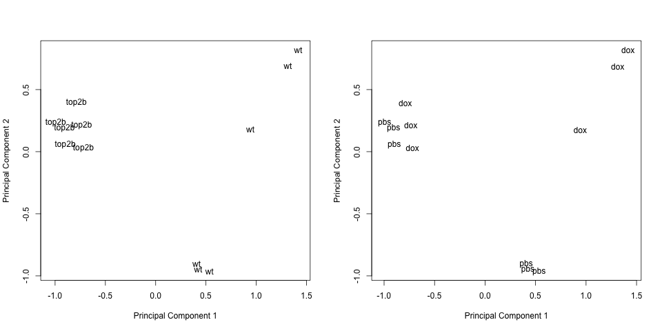
# Plot delle componenti principali etichettate per genotipo
plotMDS(eset, labels = pData(eset)[, "genotype"], gene.selection = "common")
# Plot delle componenti principali etichettate per trattamento
plotMDS(eset, labels = pData(eset)[, "treatment"], gene.selection = "common")

Passi per l'analisi di espressione differenziale

Crea la matrice di disegno con model.matrix
Costruisci la matrice dei contrasti con makeContrasts
Testa i contrasti con lmFit, contrasts.fit ed eBayes

Modello a medie di gruppo per lo studio con doxorubicina

$$ Y = \beta_1 X_1 + \beta_2 X_2 + \beta_3 X_3 + \beta_4 X_4 + \epsilon $$

$\beta_1$ - Livello medio di espressione in topi top2b trattati con dox
$\beta_2$ - Livello medio di espressione in top2b trattati con pbs
$\beta_3$ - Livello medio di espressione in topi wt trattati con dox
$\beta_4$ - Livello medio di espressione in wt trattati con pbs

Contrasti per lo studio con doxorubicina

	$\beta_1$	$\beta_2$	$\beta_3$	$\beta_4$
`genotype`	top2b	top2b	wt	wt
`treatment`	dox	pbs	dox	pbs

Response of wild type mice to dox treatment: $\beta_3 - \beta_4 = 0$
Response of Top2b null mice to dox treatment: $\beta_1 - \beta_2 = 0$
Differences between Top2b null and wild type mice in response to dox treatment: $(\beta_1 - \beta_2) - (\beta_3 - \beta_4) = 0$

Test dello studio con doxorubicina

Stima i coefficienti del modello con lmFit
Applica i contrasti con contrasts.fit
Calcola le t-statistiche con eBayes

# Riassumi i risultati
results <- decideTests(fit2)
summary(results)

# Crea un diagramma di Venn
vennDiagram(results)

Esercitiamoci!

Analisi dell'espressione differenziale con limma in R