Personalizzare le opzioni di tigris

Analizzare i dati del Censimento USA in R

Kyle Walker

Instructor

Cartographic boundary shapefiles

Gli shapefile TIGER/Line includono le aree d'acqua delle entità
- Possono non essere adatti alla mappatura tematica
Alternativa: cartographic boundary shapefiles
- Disponibili in tigris con l'argomento cb = TRUE

File TIGER/Line vs. cartographic boundary

ri_tiger <- counties("RI")
ri_cb <- counties("RI", cb = TRUE)

par(mfrow = c(1, 2))
plot(ri_tiger, main = "TIGER/Line")
plot(ri_cb, main = "Cartographic boundary")

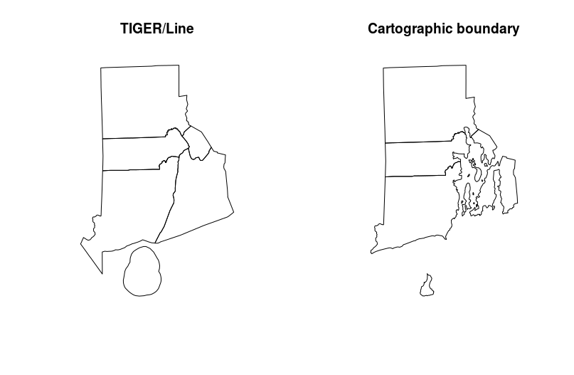
Confronto Rhode Island

tigris e simple features

options(tigris_class = "sf")
az_sf <- counties("AZ", cb = TRUE)
class(az_sf)

"sf"         "data.frame"

st_geometry(az_sf)

Geometry set for 15 features 
geometry type:  MULTIPOLYGON
dimension:      XY
bbox:           xmin: -114.8165 ymin: 31.33218 xmax: -109.0452 ymax: 37.00426
epsg (SRID):    4269
proj4string:    +proj=longlat +datum=NAD83 +no_defs

Caching dei dati tigris

Aspettare il download di grandi shapefile del Census può essere noioso!
Alternativa: options(tigris_use_cache = TRUE)
Per impostare la cartella cache: funzione tigris_cache_dir()

Dati storici e tigris

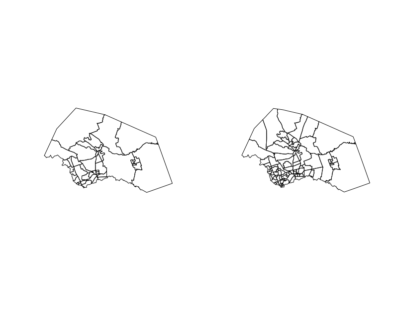
In tigris puoi ottenere dati storici con il parametro year
Dati disponibili per 1990, 2000, 2010 e 2011-2017

williamson90 <- tracts(state = "TX", county = "Williamson", 
                       cb = TRUE, year = 1990)

williamson16 <- tracts(state = "TX", county = "Williamson", 
                       cb = TRUE, year = 2016)

par(mfrow = c(1, 2))
plot(williamson90$geometry)
plot(williamson16$geometry)

Confronto Williamson County

Esercitiamoci!

Analizzare i dati del Censimento USA in R