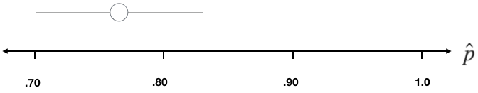
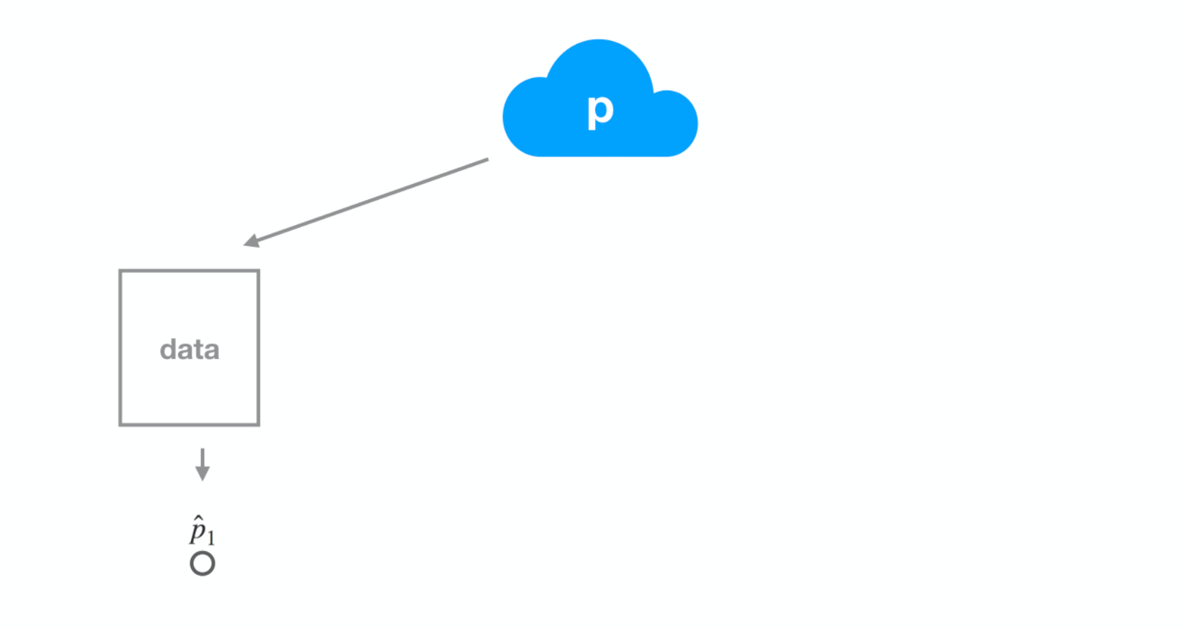
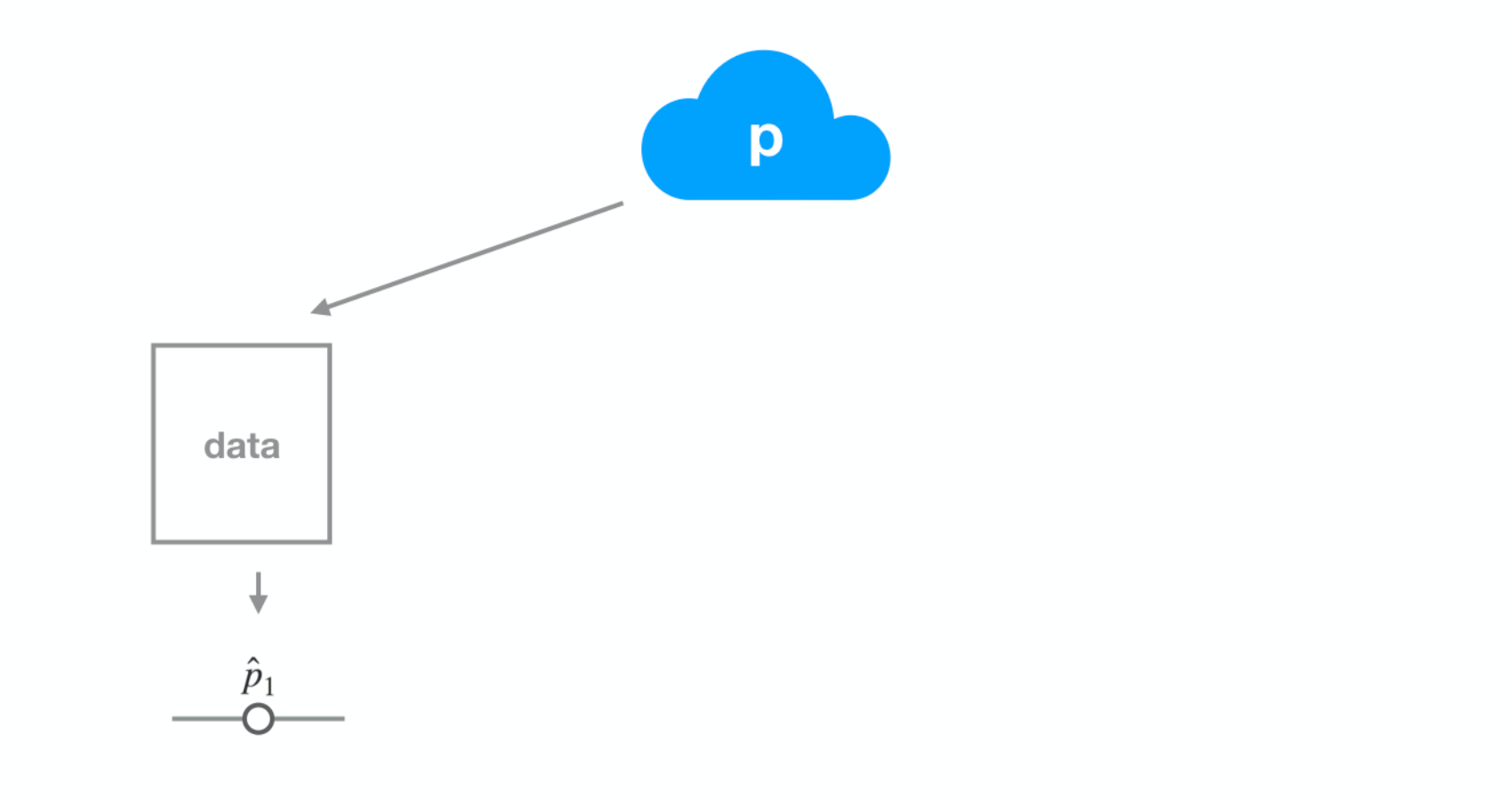
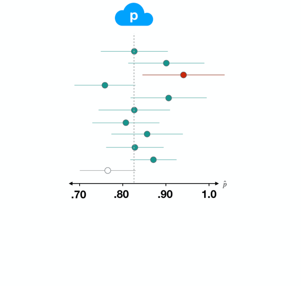
Interpretare un intervallo di confidenza
Inferenza per dati categorici in R

Andrew Bray
Assistant Professor of Statistics at Reed College
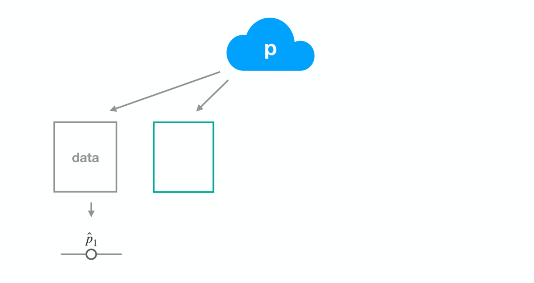
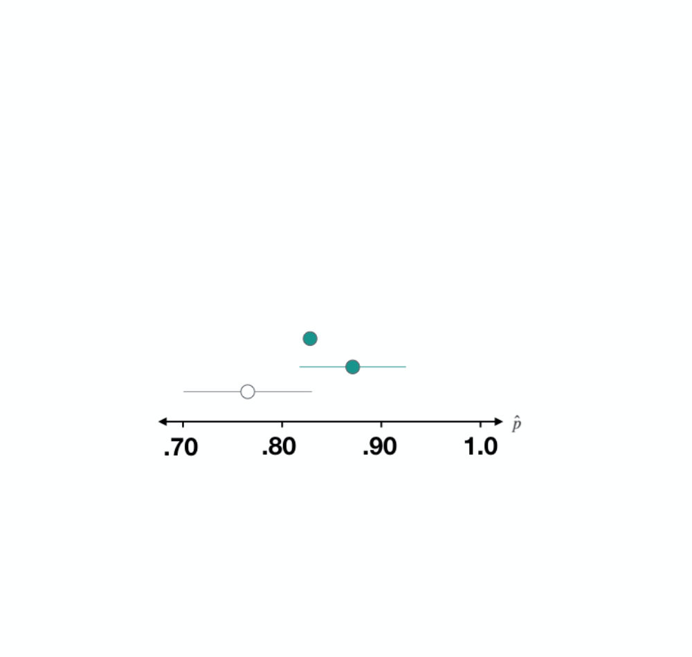
Dataset 1

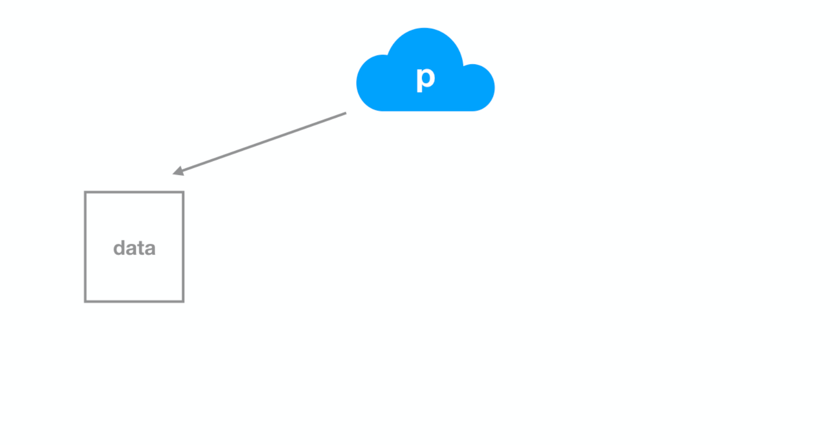
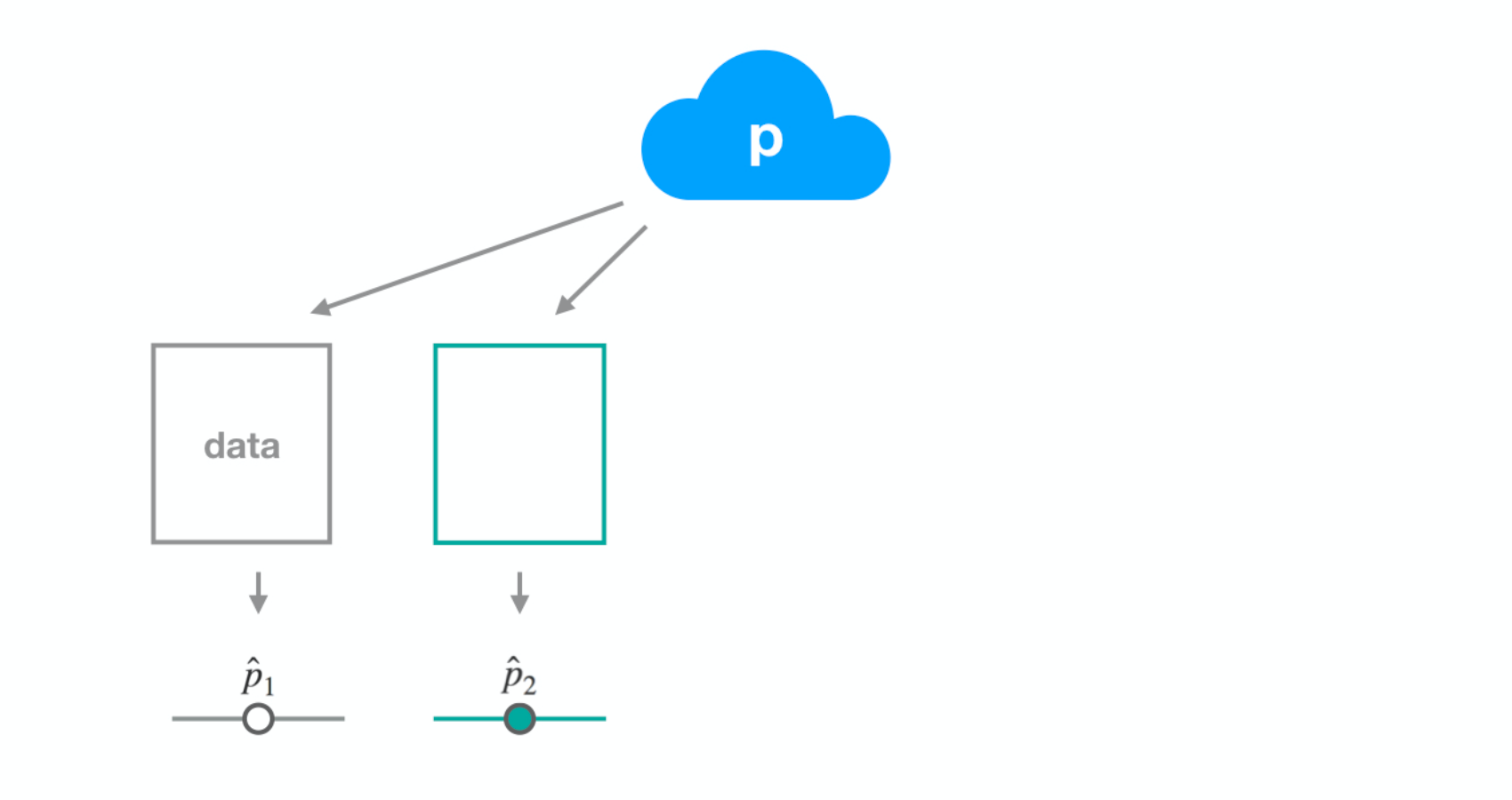
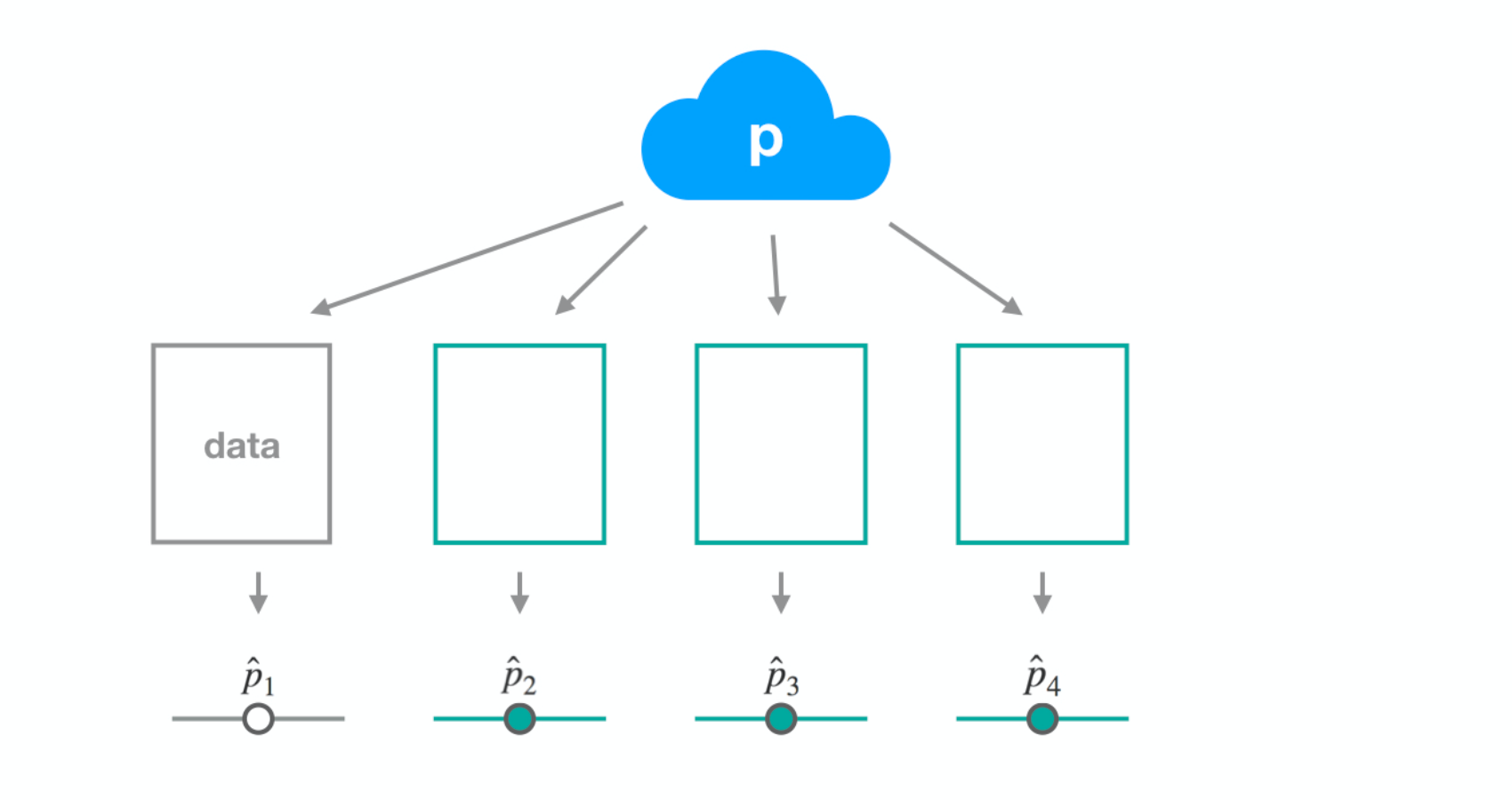
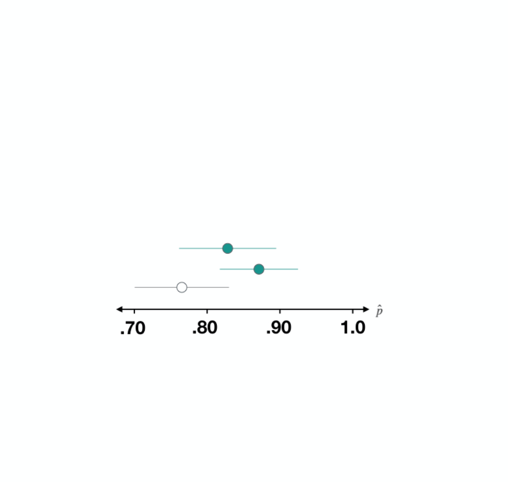
Dataset 2
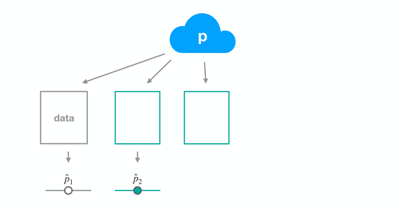
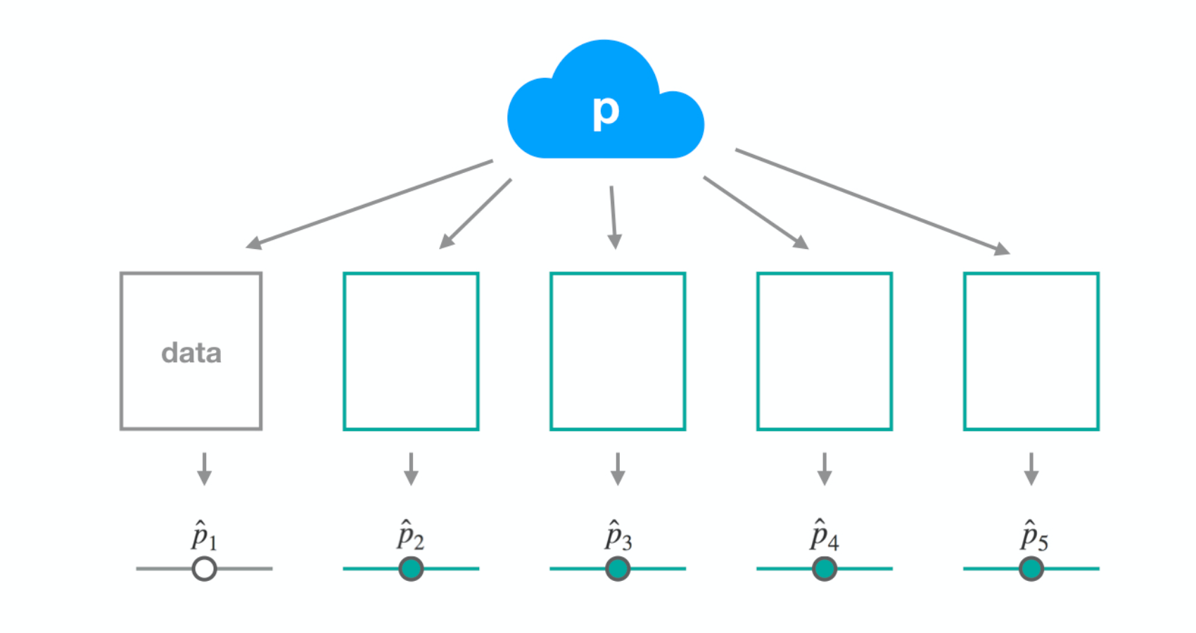
Dataset 3
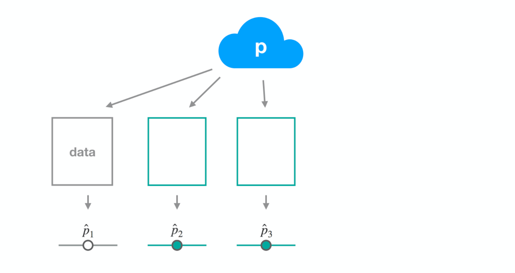
Dataset 3
Dataset 3
Dataset 3
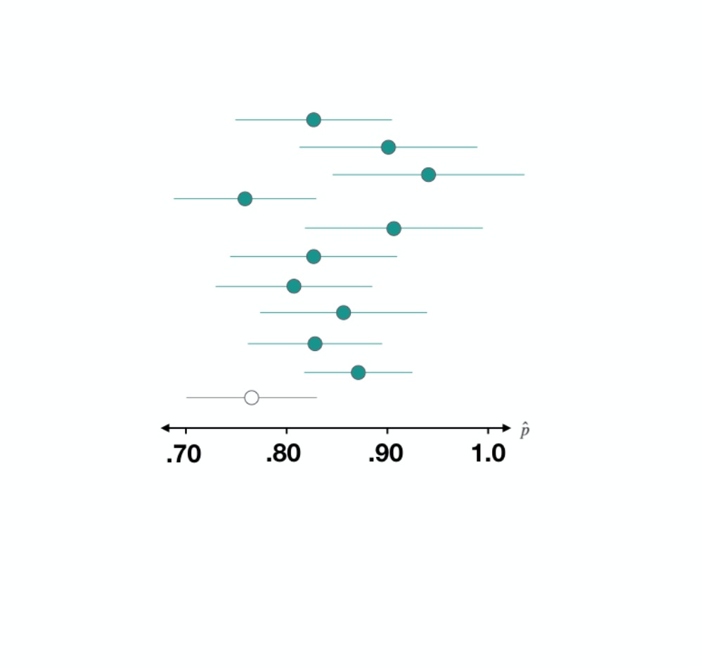
Dataset 3
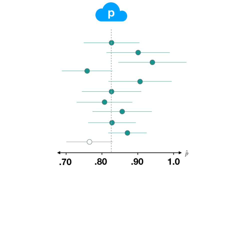
Dataset 3
Inferenza per dati categorici in R
Andrew Bray
Assistant Professor of Statistics at Reed College

