Casi di studio: analisi di reti in R
Edmund Hart
Instructor
library(HiveR)
library(igraph)

# Crea un grafo casuale
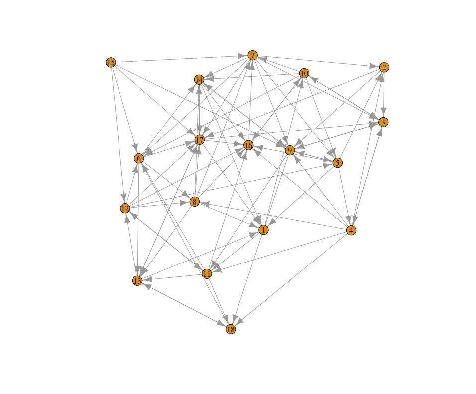
rand_g <- erdos.renyi.game(18, 0.3, "gnp", directed = TRUE)

# Disegna il grafo casuale
plot(rand_g, vertex.size = 7)
# Converti in dataframe per hive plot e aggiungi pesi
rand_g_df <- as.data.frame(get.edgelist(rand_g))
rand_g_df$weight <- 1

# Converti in oggetto hive
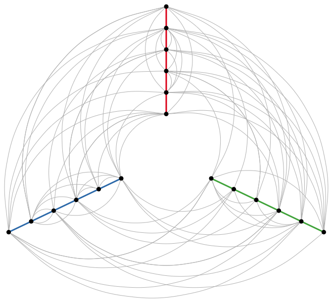
rand_hive <- edge2HPD(edge_df = rand_g_df)

# Imposta asse e raggio di ogni nodo
rand_hive$nodes$axis <- sort(rep(1:3, 6))
rand_hive$nodes$radius <- as.double(rep(1:6, 3))
# Converti in dataframe per hive plot e aggiungi pesi rand_g_df <- as.data.frame(get.edgelist(rand_g)) rand_g_df$weight <- 1
# Converti in oggetto hive rand_hive <- edge2HPD(edge_df = rand_g_df)
# Imposta asse e raggio di ogni nodo rand_hive$nodes$axis <- sort(rep(1:3, 6)) rand_hive$nodes$radius <- as.double(rep(1:6, 3))
# Vedi come cambiano i nodi
rand_hive$nodes
id lab axis radius size color
1   2    1      1    1 black
2   8    1      2    1 black
3   9    1      3    1 black
4   3    1      4    1 black
5   4    1      5    1 black
6   7    1      6    1 black
7  11    2      1    1 black
8  14    2      2    1 black
9  18    2      3    1 black
# Mostra l'hive plot
plotHive(rand_hive, method = "abs", bkgnd = "white")
# Imposta la posizione di ogni nodo
rand_hive$nodes$axis <- sort(rep(1:3, 6))
rand_hive$nodes$radius <- as.double(rep(1:6, 3))

# Aggiungi pesi a ogni arco
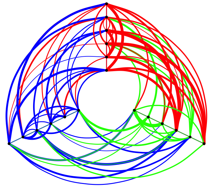
rand_hive$edges$weight <- as.double(
                      rpois(length(rand_hive$edges$weight), 5)
                          )

# Colora in base all'origine dell'arco
rand_hive$edges$color[rand_hive$edges$id1 %in% 1:6] <- 'red'
rand_hive$edges$color[rand_hive$edges$id1 %in% 7:12] <- 'blue'
rand_hive$edges$color[rand_hive$edges$id1 %in% 13:18] <- 'green'

# Disegna
plotHive(rand_hive, method = "abs", bkgnd = "white")
# Imposta la posizione di ogni nodo rand_hive$nodes$axis <- sort(rep(1:3, 6)) rand_hive$nodes$radius <- as.double(rep(1:6, 3))
# Aggiungi pesi a ogni arco rand_hive$edges$weight <- as.double( rpois(length(rand_hive$edges$weight), 5) ) # Colora in base all'origine dell'arco rand_hive$edges$color[rand_hive$edges$id1 %in% 1:6] <- 'red' rand_hive$edges$color[rand_hive$edges$id1 %in% 7:12] <- 'blue' rand_hive$edges$color[rand_hive$edges$id1 %in% 13:18] <- 'green'
# Disegna plotHive(rand_hive, method = "abs", bkgnd = "white")
# Crea un grafo casuale
rand_g <- erdos.renyi.game(10, 0.3, "gnp", directed = FALSE)
rand_g <- simplify(rand_g)

# Aggiungi nomi ai vertici
V(rand_g)$name <- LETTERS[1:length(V(rand_g))]

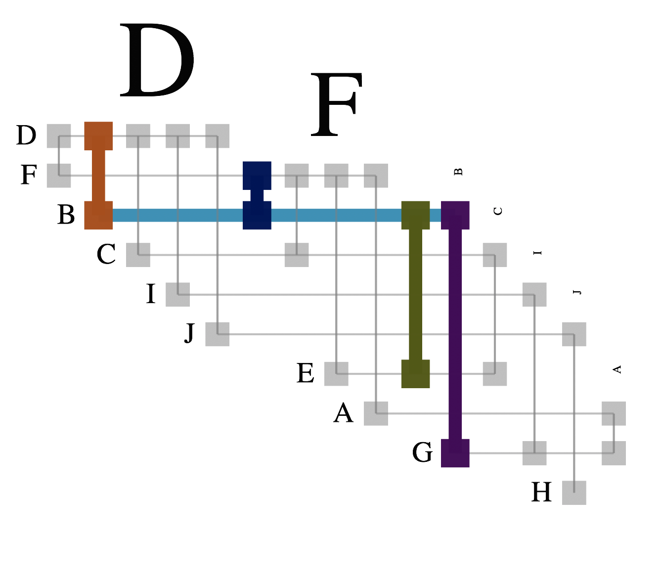
# Crea un biofabric plot
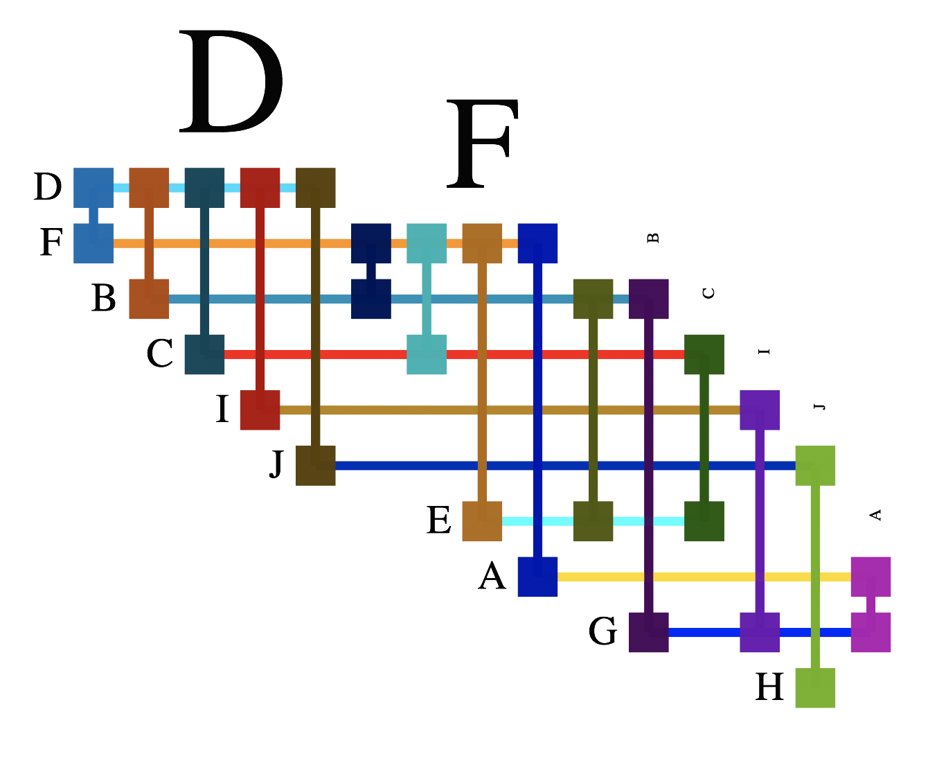
biofbc <- bioFabric(rand_g)
bioFabric_htmlwidget(biofbc)
# Crea un grafo casuale rand_g <- erdos.renyi.game(10, 0.3, "gnp", directed = FALSE) rand_g <- simplify(rand_g)
# Aggiungi nomi ai vertici V(rand_g)$name <- LETTERS[1:length(V(rand_g))]
# Crea un biofabric plot biofbc <- bioFabric(rand_g) bioFabric_htmlwidget(biofbc)