Lavorare con un oggetto di forecast

Progettare pipeline di forecasting per la produzione

Rami Krispin

Senior Manager, Data Science and Engineering

Lavora con un oggetto di forecast

Preparazione dati
Allena e testa più modelli di forecast
Valuta le prestazioni dei modelli
Il pacchetto statsforecast
- mlforecast negli esercizi

Partizione di training

Serie temporale

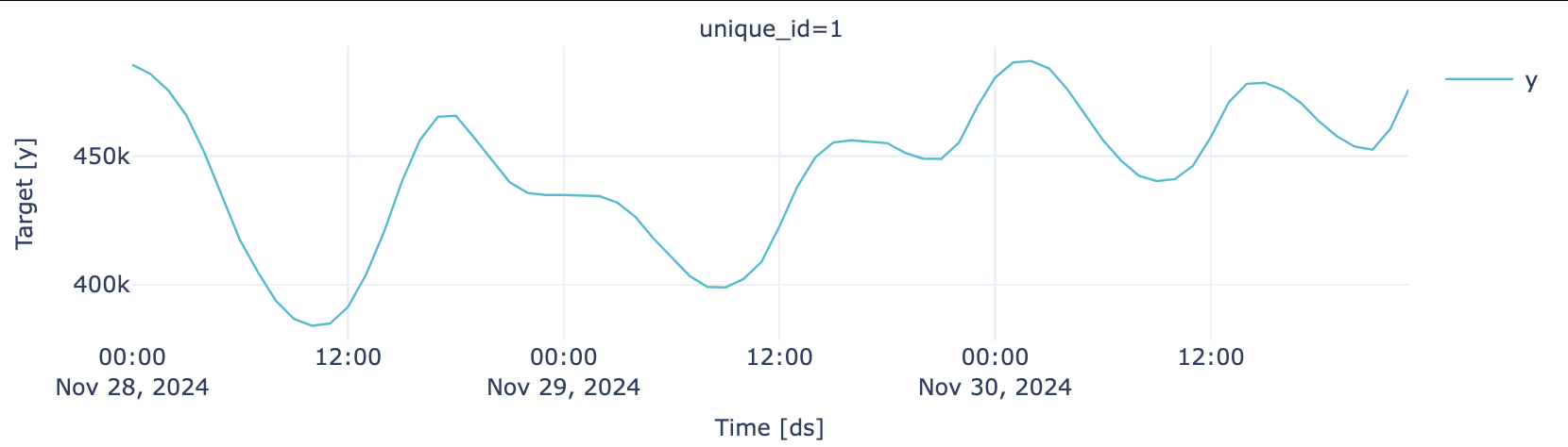
Partizione di test

Librerie richieste

import pandas as pd 
import datetime

Librerie richieste

from statsforecast import StatsForecast

from statsforecast.models import (
    DynamicOptimizedTheta,
    SeasonalNaive,
    AutoARIMA,
    HoltWinters,
    MSTL
)

from utilsforecast.plotting import plot_series

Formato dati di statsforecast

Formato input dati:

unique_id - ID della serie
ds - timestamp della serie
y - valori della serie

Preparazione dati - caricamento

ts = pd.read_csv("data/data.csv")
ts["ds"] = pd.to_datetime(ts["ds"])
ts = ts.sort_values("ds")
ts = ts[["unique_id", "ds", "y"]]

os.environ['NIXTLA_ID_AS_COL'] = '1'

 unique_id        ds             y
0    1    2022-11-11 23:00:00    456403
1    1    2022-11-12 00:00:00    458842
2    1    2022-11-12 01:00:00    455111
3    1    2022-11-12 02:00:00    448035
4    1    2022-11-12 03:00:00    438165

Preparazione dati - split train/test

Dividi la serie in train e test
- usando datetime.timedelta
- lascia le ultime 72 ore per il test

test_length = 72

train_end = end  - datetime.timedelta(hours = test_length)

train = ts[ts["ds"] <= train_end]
test = ts[ts["ds"] > train_end]

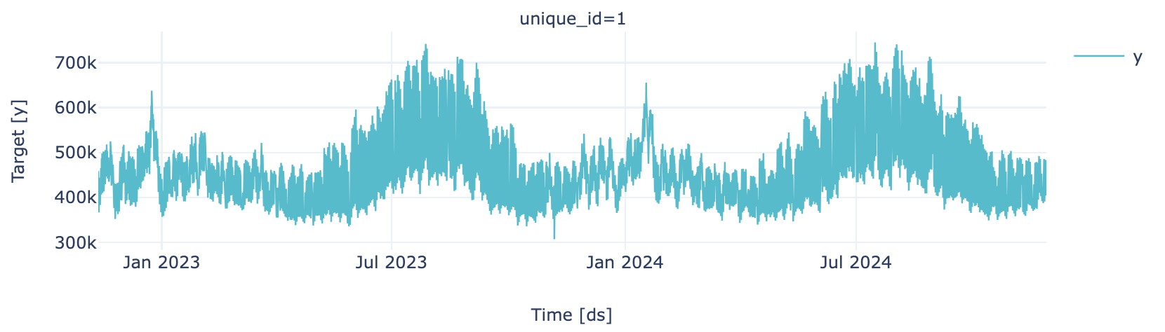
Preparazione dati

plot_series(train, engine = "plotly")

Serie temporale

plot_series(test, engine = "plotly")

Partizione di test

Previsioni con StatsModels

# Istanzia modelli con stagionalità oraria
auto_arima = AutoARIMA()
s_naive = SeasonalNaive(season_length=24)
theta =  DynamicOptimizedTheta(season_length=24)


# Istanzia modelli con stagionalità oraria e settimanale
mstl1 = MSTL(season_length=[24, 24 * 7], 
            trend_forecaster=AutoARIMA(),
            alias="MSTL_ARIMA_trend")

mstl2 = MSTL(season_length=[24, 24 * 7], 
            trend_forecaster=HoltWinters(),
            alias="MSTL_Holt_trend")

Previsioni con StatsModels

# Combina i modelli in una lista
stats_models = [auto_arima, s_naive, theta, mstl1, mstl2]


# Istanzia l'oggetto modello
sf = StatsForecast( 
    models=stats_models,
    freq="h", 
    fallback_model = AutoARIMA(),
    n_jobs= -1)

Previsioni con StatsModels

# Combina i modelli in una lista
stats_models = [auto_arima, s_naive, theta, mstl1, mstl2]


# Istanzia l'oggetto modello
sf = StatsForecast( 
    models=stats_models,
    freq="h", 
    fallback_model = AutoARIMA(),
    n_jobs= -1)


# Crea il forecast
forecast_stats = sf.forecast(df=train, h=72, level=[95])

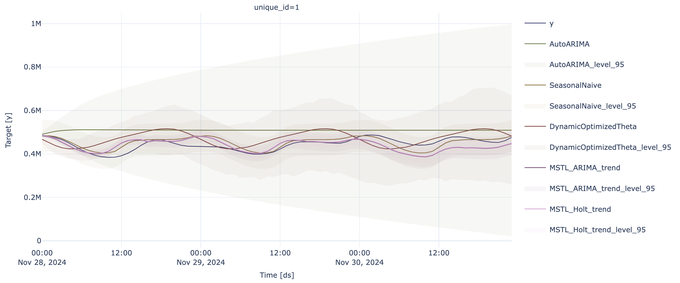
Previsioni con StatsModels

p = sf.plot(test, forecast_stats, engine = "plotly", level=[95])
p.update_layout(height=400)

Grafico del forecast

Valutazione del modello

def mape(y, yhat):
    mape = mean(abs(y - yhat)/ y) 
    return mape

def rmse(y, yhat):
    rmse = (mean((y - yhat) ** 2 )) ** 0.5
    return rmse

def coverage(y, lower, upper):
    coverage = sum((y <= upper) & (y >= lower)) / len(y)
    return coverage

Valutazione del modello

fc = forecast_stats.merge(test, how="left", on="ds")
fc_performance = None

for i in [str(m) for m in stats_models]:
    m = mape(y = fc["y"], yhat = fc[i])
    r = rmse(y = fc["y"], yhat = fc[i])
    c = coverage(y = fc["y"], lower = fc[i + "-lo-95"], upper = fc[i + "-hi-95"])

    perf = {"model": i,
            "mape": m,
            "rmse": r,
            "coverage": c}
    if fc_performance is None:
        fc_performance = pd.DataFrame([perf])
    else:
        fc_performance = pd.concat([fc_performance, pd.DataFrame([perf])])
fc_performance.reset_index(drop=True, inplace=True)

Valutazione del modello

print(fc_performance.sort_values("rmse"))

     model                    mape        rmse            coverage
1    SeasonalNaive            0.041340    22410.483959    1.000000
4    MSTL_Holt_trend          0.053939    30201.299395    0.513889
3    MSTL_ARIMA_trend         0.053771    30428.240235    0.666667
2    DynamicOptimizedTheta    0.090566    45189.869437    0.916667
0    AutoARIMA                0.149790    70483.617198    1.000000

Valutazione del modello

print(fc_performance.sort_values("rmse"))

     model                    mape        rmse            coverage
1    SeasonalNaive            0.041340    22410.483959    1.000000
4    MSTL_Holt_trend          0.053939    30201.299395    0.513889
3    MSTL_ARIMA_trend         0.053771    30428.240235    0.666667
2    DynamicOptimizedTheta    0.090566    45189.869437    0.916667
0    AutoARIMA                0.149790    70483.617198    1.000000

Possiamo migliorare i risultati?

Impostazioni diverse per più accuratezza
Gli esperimenti aiutano

Passons à la pratique !

Progettare pipeline di forecasting per la produzione