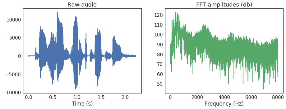
The spectrogram - spectral changes to sound over time

Machine Learning cho Dữ liệu Chuỗi thời gian bằng Python

Chris Holdgraf

Fellow, Berkeley Institute for Data Science

Fourier transforms

Timeseries data can be described as a combination of quickly-changing things and slowly-changing things
At each moment in time, we can describe the relative presence of fast- and slow-moving components
The simplest way to do this is called a Fourier Transform
This converts a single timeseries into an array that describes the timeseries as a combination of oscillations

A Fourier Transform (FFT)

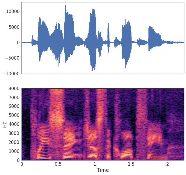
Spectrograms: combinations of windows Fourier transforms

A spectrogram is a collection of windowed Fourier transforms over time
Similar to how a rolling mean was calculated:
1. Choose a window size and shape
2. At a timepoint, calculate the FFT for that window
3. Slide the window over by one
4. Aggregate the results
Called a Short-Time Fourier Transform (STFT)

Calculating the STFT

We can calculate the STFT with librosa
There are several parameters we can tweak (such as window size)
For our purposes, we'll convert into decibels which normalizes the average values of all frequencies
We can then visualize it with the specshow() function

Calculating the STFT with code

# Import the functions we'll use for the STFT
from librosa.core import stft, amplitude_to_db
from librosa.display import specshow
import matplotlib.pyplot as plt

# Calculate our STFT
HOP_LENGTH = 2**4
SIZE_WINDOW = 2**7
audio_spec = stft(audio, hop_length=HOP_LENGTH, n_fft=SIZE_WINDOW)

# Convert into decibels for visualization
spec_db = amplitude_to_db(audio_spec)

# Visualize
fig, ax = plt.subplots()
specshow(spec_db, sr=sfreq, x_axis='time', 
         y_axis='hz', hop_length=HOP_LENGTH, ax=ax)

Spectral feature engineering

Each timeseries has a different spectral pattern.
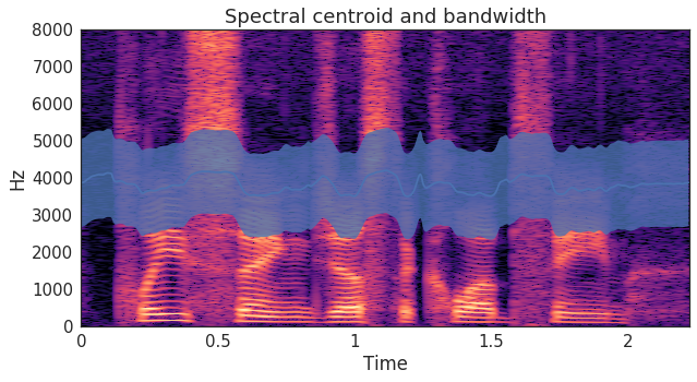
We can calculate these spectral patterns by analyzing the spectrogram.
For example, spectral bandwidth and spectral centroids describe where most of the energy is at each moment in time

Calculating spectral features

# Calculate the spectral centroid and bandwidth for the spectrogram
bandwidths = lr.feature.spectral_bandwidth(S=spec)[0]
centroids = lr.feature.spectral_centroid(S=spec)[0]

# Display these features on top of the spectrogram
fig, ax = plt.subplots()
specshow(spec, x_axis='time', y_axis='hz', hop_length=HOP_LENGTH, ax=ax)
ax.plot(times_spec, centroids)
ax.fill_between(times_spec, centroids - bandwidths / 2, 
                centroids + bandwidths / 2, alpha=0.5)

Combining spectral and temporal features in a classifier

centroids_all = []
bandwidths_all = []
for spec in spectrograms:
    bandwidths = lr.feature.spectral_bandwidth(S=lr.db_to_amplitude(spec))
    centroids = lr.feature.spectral_centroid(S=lr.db_to_amplitude(spec))
    # Calculate the mean spectral bandwidth
    bandwidths_all.append(np.mean(bandwidths))  
    # Calculate the mean spectral centroid
    centroids_all.append(np.mean(centroids))  

# Create our X matrix
X = np.column_stack([means, stds, maxs, tempo_mean, 
                     tempo_max, tempo_std, bandwidths_all, centroids_all])

Let's practice!

Machine Learning cho Dữ liệu Chuỗi thời gian bằng Python