Làm việc với đối tượng dự báo

Thiết kế Pipeline Dự báo cho Môi trường Production

Rami Krispin

Senior Manager, Data Science and Engineering

Làm việc với đối tượng dự báo

Chuẩn bị dữ liệu
Huấn luyện và kiểm tra nhiều mô hình dự báo
Đánh giá hiệu suất mô hình
Gói statsforecast
- mlforecast trong bài tập

Tập huấn luyện

Chuỗi thời gian

Tập kiểm tra

Thư viện cần thiết

import pandas as pd 
import datetime

Thư viện cần thiết

from statsforecast import StatsForecast

from statsforecast.models import (
    DynamicOptimizedTheta,
    SeasonalNaive,
    AutoARIMA,
    HoltWinters,
    MSTL
)

from utilsforecast.plotting import plot_series

Định dạng dữ liệu cho statsforecast

Định dạng đầu vào:

unique_id - ID chuỗi
ds - mốc thời gian
y - giá trị chuỗi

Chuẩn bị dữ liệu - nạp dữ liệu

ts = pd.read_csv("data/data.csv")
ts["ds"] = pd.to_datetime(ts["ds"])
ts = ts.sort_values("ds")
ts = ts[["unique_id", "ds", "y"]]

os.environ['NIXTLA_ID_AS_COL'] = '1'

 unique_id        ds             y
0    1    2022-11-11 23:00:00    456403
1    1    2022-11-12 00:00:00    458842
2    1    2022-11-12 01:00:00    455111
3    1    2022-11-12 02:00:00    448035
4    1    2022-11-12 03:00:00    438165

Chuẩn bị dữ liệu - tách train/test

Chia chuỗi thời gian thành tập huấn luyện và kiểm tra
- dùng datetime.timedelta
- giữ 72 giờ cuối làm kiểm tra

test_length = 72

train_end = end  - datetime.timedelta(hours = test_length)

train = ts[ts["ds"] <= train_end]
test = ts[ts["ds"] > train_end]

Chuẩn bị dữ liệu

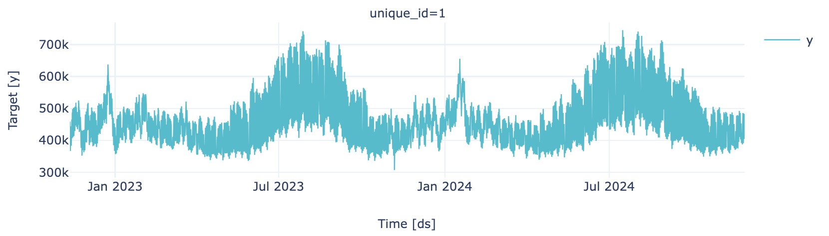
plot_series(train, engine = "plotly")

Chuỗi thời gian

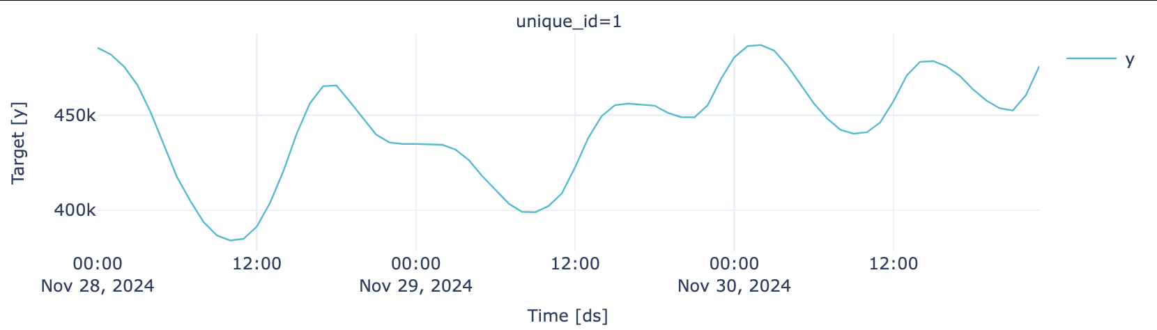
plot_series(test, engine = "plotly")

Tập kiểm tra

Dự báo với StatsModels

# Khởi tạo mô hình với mùa vụ theo giờ
auto_arima = AutoARIMA()
s_naive = SeasonalNaive(season_length=24)
theta =  DynamicOptimizedTheta(season_length=24)


# Khởi tạo mô hình với mùa vụ theo giờ và theo tuần
mstl1 = MSTL(season_length=[24, 24 * 7], 
            trend_forecaster=AutoARIMA(),
            alias="MSTL_ARIMA_trend")

mstl2 = MSTL(season_length=[24, 24 * 7], 
            trend_forecaster=HoltWinters(),
            alias="MSTL_Holt_trend")

Dự báo với StatsModels

# Gộp mô hình vào một danh sách
stats_models = [auto_arima, s_naive, theta, mstl1, mstl2]


# Khởi tạo đối tượng mô hình
sf = StatsForecast( 
    models=stats_models,
    freq="h", 
    fallback_model = AutoARIMA(),
    n_jobs= -1)

Dự báo với StatsModels

# Gộp mô hình vào một danh sách
stats_models = [auto_arima, s_naive, theta, mstl1, mstl2]


# Khởi tạo đối tượng mô hình
sf = StatsForecast( 
    models=stats_models,
    freq="h", 
    fallback_model = AutoARIMA(),
    n_jobs= -1)


# Tạo dự báo
forecast_stats = sf.forecast(df=train, h=72, level=[95])

Dự báo với StatsModels

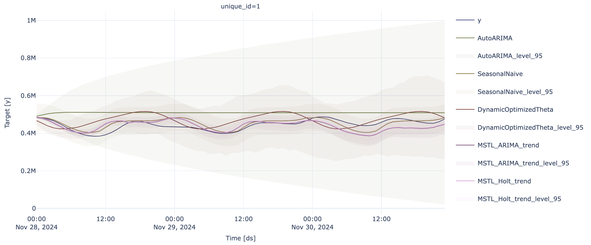
p = sf.plot(test, forecast_stats, engine = "plotly", level=[95])
p.update_layout(height=400)

Biểu đồ dự báo

Đánh giá mô hình

def mape(y, yhat):
    mape = mean(abs(y - yhat)/ y) 
    return mape

def rmse(y, yhat):
    rmse = (mean((y - yhat) ** 2 )) ** 0.5
    return rmse

def coverage(y, lower, upper):
    coverage = sum((y <= upper) & (y >= lower)) / len(y)
    return coverage

Đánh giá mô hình

fc = forecast_stats.merge(test, how="left", on="ds")
fc_performance = None

for i in [str(m) for m in stats_models]:
    m = mape(y = fc["y"], yhat = fc[i])
    r = rmse(y = fc["y"], yhat = fc[i])
    c = coverage(y = fc["y"], lower = fc[i + "-lo-95"], upper = fc[i + "-hi-95"])

    perf = {"model": i,
            "mape": m,
            "rmse": r,
            "coverage": c}
    if fc_performance is None:
        fc_performance = pd.DataFrame([perf])
    else:
        fc_performance = pd.concat([fc_performance, pd.DataFrame([perf])])
fc_performance.reset_index(drop=True, inplace=True)

Đánh giá mô hình

print(fc_performance.sort_values("rmse"))

     model                    mape        rmse            coverage
1    SeasonalNaive            0.041340    22410.483959    1.000000
4    MSTL_Holt_trend          0.053939    30201.299395    0.513889
3    MSTL_ARIMA_trend         0.053771    30428.240235    0.666667
2    DynamicOptimizedTheta    0.090566    45189.869437    0.916667
0    AutoARIMA                0.149790    70483.617198    1.000000

Đánh giá mô hình

print(fc_performance.sort_values("rmse"))

     model                    mape        rmse            coverage
1    SeasonalNaive            0.041340    22410.483959    1.000000
4    MSTL_Holt_trend          0.053939    30201.299395    0.513889
3    MSTL_ARIMA_trend         0.053771    30428.240235    0.666667
2    DynamicOptimizedTheta    0.090566    45189.869437    0.916667
0    AutoARIMA                0.149790    70483.617198    1.000000

Có thể cải thiện kết quả không?

Điều chỉnh tham số để tăng độ chính xác
Cần chạy thử nghiệm

Ayo berlatih!

Thiết kế Pipeline Dự báo cho Môi trường Production