Mô hình phân loại

Mô hình hóa với tidymodels trong R

David Svancer

Data Scientist

Dự đoán mua hàng

Mô hình phân loại dự đoán biến kết quả dạng phân loại

Dự đoán hành vi mua hàng

purchased	total_time	total_visits
yes	800	3
yes	978	7
no	220	4
no	124	5
yes	641	4

Biểu đồ phân loại

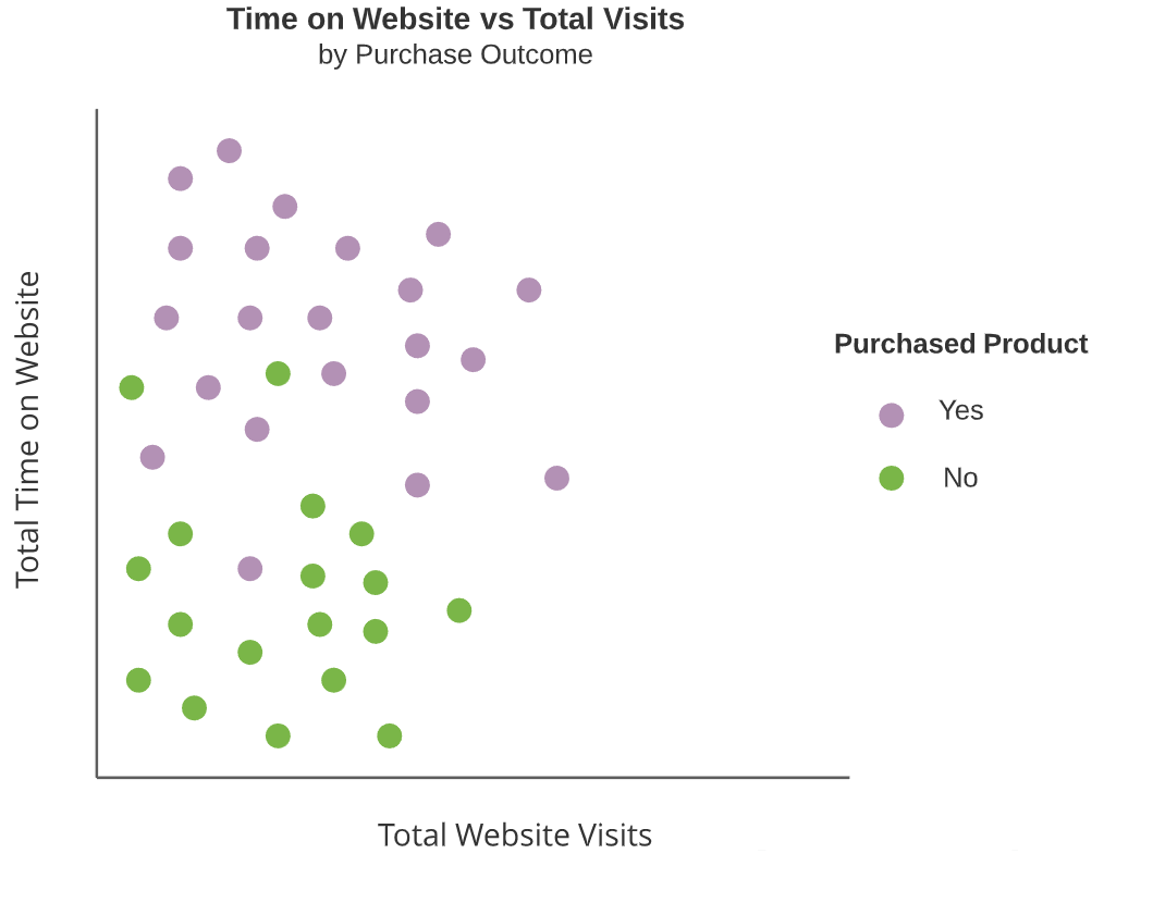
Thuật toán phân loại

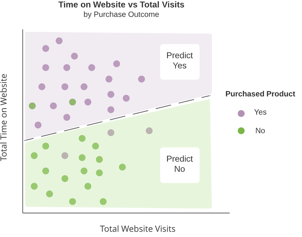
Mục tiêu: Tạo các vùng riêng, không chồng lấn theo giá trị biến dự báo

Dự đoán cùng một kết quả phân loại trong mỗi vùng

Biểu đồ phân loại

Thuật toán phân loại

Mục tiêu: Tạo các vùng riêng, không chồng lấn theo giá trị biến dự báo

Dự đoán cùng một kết quả phân loại trong mỗi vùng

Hồi quy logistic

Thuật toán phân loại phổ biến tạo ranh giới tách tuyến tính giữa các hạng mục

Phân loại với ranh giới

Dữ liệu chấm điểm lead

leads_df

# A tibble: 1,328 x 7
   purchased total_visits total_time pages_per_visit total_clicks lead_source    us_location
   <fct>            <dbl>      <dbl>           <dbl>        <dbl> <fct>          <fct>      
 1 yes                  7       1148            7              59 direct_traffic west       
 2 no                   8        100            2.67           24 direct_traffic west       
 3 no                   5        228            2.5            25 email          southeast  
 4 no                   7        481            2.33           21 organic_search west       
 5 no                   4        177            4              37 direct_traffic west       
 6 no                   2       1273            2              26 email          midwest    
 7 no                   3        711            3              28 organic_search west       
 8 no                   3        166            3              32 direct_traffic southeast  
 9 no                   3          7            3              23 organic_search west       
10 no                   6        562            6              48 organic_search southeast  
# ... with 1,318 more rows

Lấy mẫu lại dữ liệu

Bước đầu khi huấn luyện mô hình

Tạo đối tượng chia dữ liệu với initial_split()
Tạo tập huấn luyện và kiểm tra với training() và testing()

leads_split <- initial_split(leads_df, 
                             prop = 0.75,
                             strata = purchased)


leads_training <- leads_split %>% 
  training()


leads_test <- leads_split %>% 
  testing()

Đặc tả mô hình hồi quy logistic

Đặc tả mô hình trong parsnip

logistic_reg()
- Giao diện chung cho hồi quy logistic trong parsnip
- Engine thường dùng: 'glm'
- Chế độ: 'classification'

logistic_model <- logistic_reg() %>% 

  set_engine('glm') %>%

  set_mode('classification')

Huấn luyện mô hình

Sau khi đặc tả, dùng fit() để huấn luyện

Truyền đối tượng mô hình vào fit()
Chỉ định công thức mô hình
Cung cấp dữ liệu huấn luyện qua data

logistic_fit <- logistic_model %>% 

  fit(purchased ~ total_visits + total_time,

      data = leads_training)

Dự đoán nhãn kết quả

Hàm predict()

new_data chỉ định dữ liệu cần dự đoán
type
- 'class' trả về dự đoán phân loại

Đầu ra chuẩn hóa từ predict()

Trả về một tibble
Khi type là 'class', trả về cột factor tên .pred_class

class_preds <- logistic_fit %>%

  predict(new_data = leads_test,

          type = 'class')


class_preds

# A tibble: 332 x 1
   .pred_class
   <fct>      
 1 no         
 2 yes        
 3 no         
 4 no         
 5 yes 
 # ... with 327 more rows

Xác suất ước tính

Đặt type là 'prob' để nhận xác suất ước tính cho từng hạng mục kết quả

predict() sẽ trả về một tibble nhiều cột

Mỗi cột cho một hạng mục của biến kết quả
Quy ước tên: .pred_{outcome_category}

prob_preds <- logistic_fit %>%
  predict(new_data = leads_test,
          type = 'prob')

prob_preds

# A tibble: 332 x 2
   .pred_yes .pred_no
       <dbl>    <dbl>
 1    0.134     0.866
 2    0.729     0.271
 3    0.133     0.867
 4    0.0916    0.908
 5    0.598     0.402
# ... with 327 more rows

Kết hợp kết quả

Để đánh giá mô hình với gói yardstick, cần một tibble kết quả

Có thể ghép biến kết quả từ tập kiểm tra và các tibble dự đoán bằng bind_cols()

leads_results <- leads_test %>% 
  select(purchased) %>% 
  bind_cols(class_preds, prob_preds)

leads_results

# A tibble: 332 x 4
   purchased .pred_class .pred_yes .pred_no
   <fct>     <fct>           <dbl>    <dbl>
 1 no        no             0.134     0.866
 2 yes       yes            0.729     0.271
 3 no        no             0.133     0.867
 4 no        no             0.0916    0.908
 5 yes       yes            0.598     0.402
# ... with 327 more rows

Dữ liệu viễn thông

telecom_df

# A tibble: 975 x 9
   canceled_service cellular_service avg_data_gb avg_call_mins avg_intl_mins internet_service   contract    months_with_company monthly_charges
   <fct>            <fct>               <dbl>         <dbl>        <dbl>         <fct>           <fct>               <dbl>           <dbl>
 1 yes              single_line         7.78           497         127         fiber_optic     month_to_month         7              76.4
 2 yes              single_line         9.04           336         88          fiber_optic     month_to_month         10             94.9
 3 no               single_line         10.3           262         55          fiber_optic     one_year               50             103. 
 4 yes              multiple_lines      5.08           250         107         digital         one_year               53             60.0
 5 no               multiple_lines      8.05           328         122         digital         two_year               50             75.2
 6 no               single_line         9.3            326         114         fiber_optic     month_to_month         25             95.7
 7 yes              multiple_lines      8.01           525         97          fiber_optic     month_to_month         19             83.6
 8 no               multiple_lines      9.4            312         147         fiber_optic     one_year               50             99.4
 9 yes              single_line         5.29           417         96          digital         month_to_month         8              49.8
10 no               multiple_lines      9.96           340         136         fiber_optic     month_to_month         61             106. 
# ... with 965 more rows

Ayo berlatih!

Mô hình hóa với tidymodels trong R