실험 설계에서 공변량 보정

Python으로 배우는 실험 설계

James Chapman

Curriculum Manager, DataCamp

공변량 소개

공변량: 실험 결과에 영향 가능하나 주된 관심은 아님
교란 감소에 중요
결과의 정밀도와 타당성에 영향

예시: 교수법이 시험 점수에 미치는 영향

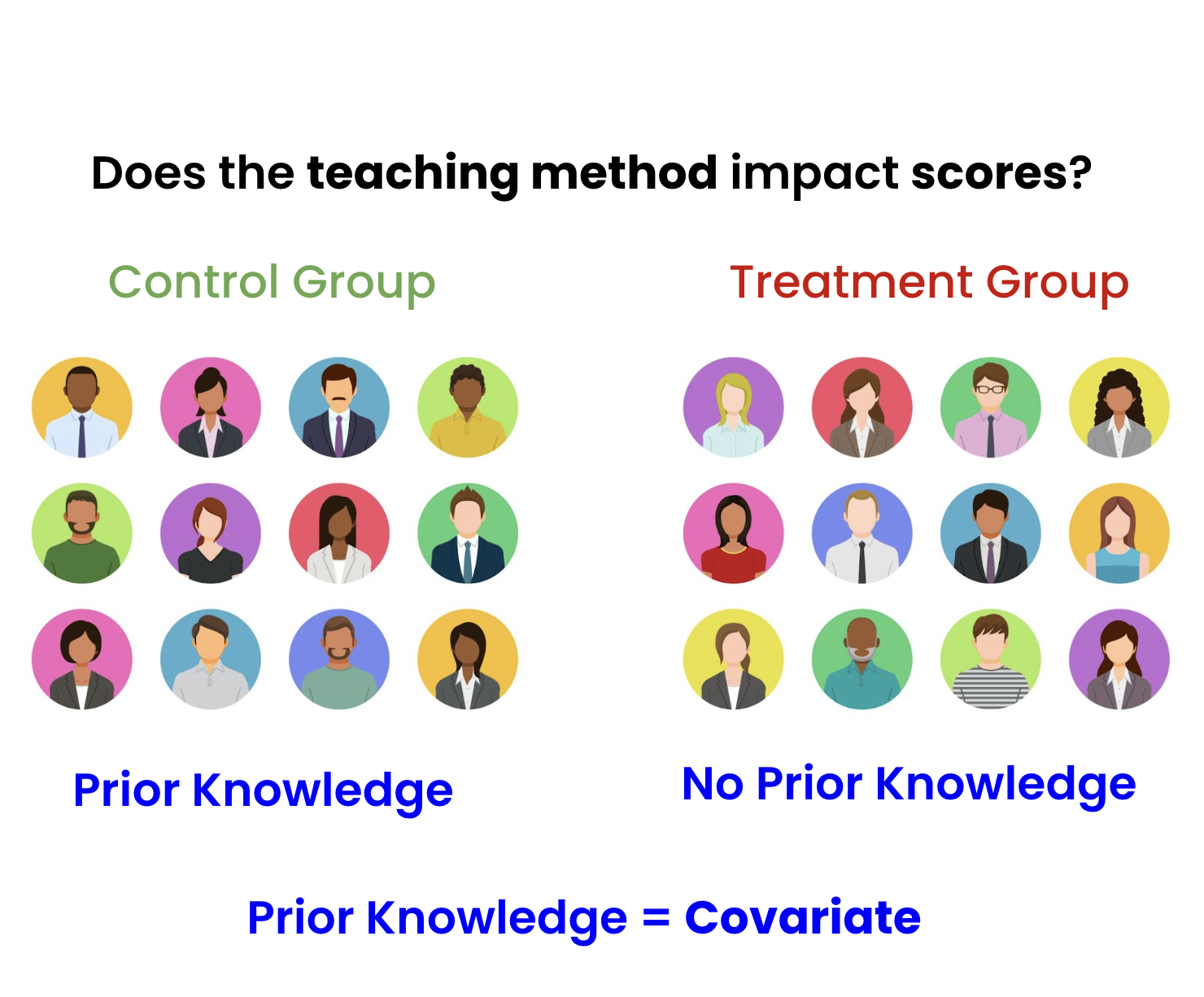
교수법이 시험 결과에 영향을 미치는지 확인하는 테스트. 두 집단의 사전 지식 분포가 불균형하여 교란을 유발하는 공변량이 됨.

실험 데이터 예시

exp_plant_data = plant_growth_data[['Plant_ID', 'Fertilizer_Type', 'Growth_cm']]

   Plant_ID  Light_Condition  Fertilizer_Type  Growth_cm
0         1    Full Sunlight        Synthetic  16.489735
1         2    Partial Shade          Organic  18.361689
2         3    Full Sunlight        Synthetic  18.039459
3         4    Full Sunlight          Organic  12.682425
4         5    Full Sunlight          Organic  21.480601

공변량 데이터 예시

covariate_data

   Plant_ID  Watering_Days_Per_Week
0         1                       6
1         2                       6
2         3                       4
3         4                       3
4         5                       7

실험 데이터와 공변량 결합

merged_plant_data = pd.merge(exp_plant_data, covariate_data, on='Plant_ID')

   Plant_ID  Fertilizer_Type  Growth_cm  Watering_Days_Per_Week
0         1        Synthetic  16.489735                       6
1         2          Organic  18.361689                       6
2         3        Synthetic  18.039459                       4
3         4          Organic  12.682425                       3
4         5          Organic  21.480601                       7

공변량 보정

from statsmodels.formula.api import ols

model = ols('Growth_cm ~ Fertilizer_Type + Watering_Days_Per_Week',
            data=merged_plant_data).fit()

model.summary()

                            OLS Regression Results                            
==============================================================================
Dep. Variable:              Growth_cm   R-squared:                       0.011
Model:                            OLS   Adj. R-squared:                 -0.006
Method:                 Least Squares   F-statistic:                    0.6370
No. Observations:                 120   Prob (F-statistic):              0.531 <---
Df Residuals:                     117   Log-Likelihood:                -360.45
Df Model:                           2   AIC:                             726.9
Covariance Type:            nonrobust   BIC:                             735.3     
==============================================================================

ANCOVA 결과 더 살펴보기

                                       coef       std err             t       P>|t|      [0.025      0.975]
<hr />-----------------------------------------------------------------------------------------------------
Intercept                           19.3373         1.150        16.820       0.000      17.060      21.614
Fertilizer_Type[T.Synthetic]        -0.2796         0.913        -0.306       0.760 <--  -2.088       1.528
Watering_Days_Per_Week               0.2507         0.229         1.097       0.275 <--  -0.202       0.703
===========================================================================================================
Omnibus:                          14.446    Durbin-Watson:                   1.992
Prob(Omnibus):                     0.001    Jarque-Bera (JB):               18.267
Skew:                              0.675    Prob(JB):                     0.000108
Kurtosis:                          4.352    Cond. No.                         13.3
==================================================================================

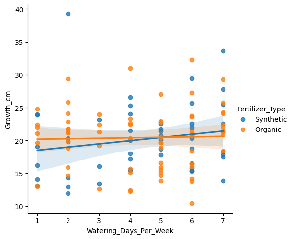
공변량 보정으로 처치 효과 시각화

import seaborn as sns
import matplotlib.pyplot as plt
sns.lmplot(x='Watering_Days_Per_Week', 
           y='Growth_cm', 
           hue='Fertilizer_Type', 
           data=merged_plant_data)
plt.show()

식물 lmplot

연습해 봅시다!

Python으로 배우는 실험 설계