ANOVA 검정

R로 하는 가설 검정

Richie Cotton

Data Evangelist at DataCamp

직업 만족도: 5가지 범주

stack_overflow %>% 
  count(job_sat)

# A tibble: 5 x 2
  job_sat                   n
  <fct>                 <int>
1 Very dissatisfied       187
2 Slightly dissatisfied   385
3 Neither                 245
4 Slightly satisfied      777
5 Very satisfied          981

다중 분포 시각화

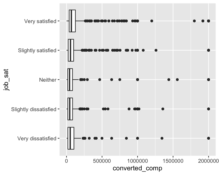
질문: 직업 만족도 수준에 따라 평균 연간 보상이 다른가요?

stack_overflow %>% 
  ggplot(aes(x = job_sat, y = converted_comp)) +
  geom_boxplot() +
  coord_flip()

5가지 범주별 보상 분포를 나타내는 상자 그림. "매우 만족"이 다른 범주보다 약간 높아 보이지만 명확하지 않습니다.

분산 분석 (ANOVA)

mdl_comp_vs_job_sat <- lm(converted_comp ~ job_sat, data = stack_overflow)

anova(mdl_comp_vs_job_sat)

Analysis of Variance Table

Response: converted_comp
            Df   Sum Sq  Mean Sq F value Pr(>F)   
job_sat      4 1.09e+12 2.73e+11    3.65 0.0057 **
Residuals 2570 1.92e+14 7.47e+10                  

Signif. codes:  0 '***' 0.001 '**' 0.01 '*' 0.05 '.' 0.1 ' ' 1

¹ lm()을 사용한 선형 회귀는 "R로 배우는 회귀 분석 입문"에서 다룹니다.

쌍별 검정

$\mu_{\text{very dissatisfied}} \neq \mu_{\text{slightly dissatisfied}}$
$\mu_{\text{very dissatisfied}} \neq \mu_{\text{neither}}$
$\mu_{\text{very dissatisfied}} \neq \mu_{\text{slightly satisfied}}$
$\mu_{\text{very dissatisfied}} \neq \mu_{\text{very satisfied}}$
$\mu_{\text{slightly dissatisfied}} \neq \mu_{\text{neither}}$

$\mu_{\text{slightly dissatisfied}} \neq \mu_{\text{slightly satisfied}}$
$\mu_{\text{slightly dissatisfied}} \neq \mu_{\text{very satisfied}}$
$\mu_{\text{neither}} \neq \mu_{\text{slightly satisfied}}$
$\mu_{\text{neither}} \neq \mu_{\text{very satisfied}}$
$\mu_{\text{slightly satisfied}} \neq \mu_{\text{very satisfied}}$

유의 수준을 $\alpha = 0.2$로 설정합니다.

pairwise.t.test()

pairwise.t.test(stack_overflow$converted_comp, stack_overflow$job_sat, p.adjust.method = "none")

    Pairwise comparisons using t tests with pooled SD 

data:  stack_overflow$converted_comp and stack_overflow$job_sat 

                      Very dissatisfied Slightly dissatisfied Neither Slightly satisfied
Slightly dissatisfied 0.26860           -                     -       -                 
Neither               0.79578           0.36858               -       -                 
Slightly satisfied    0.29570           0.82931               0.41248 -                 
Very satisfied        0.34482           0.00384               0.15939 0.00084           

P value adjustment method: none

유의미한 차이: "매우 만족" vs. "약간 불만족"; "매우 만족" vs. "보통"; "매우 만족" vs. "약간 만족"

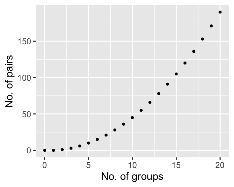
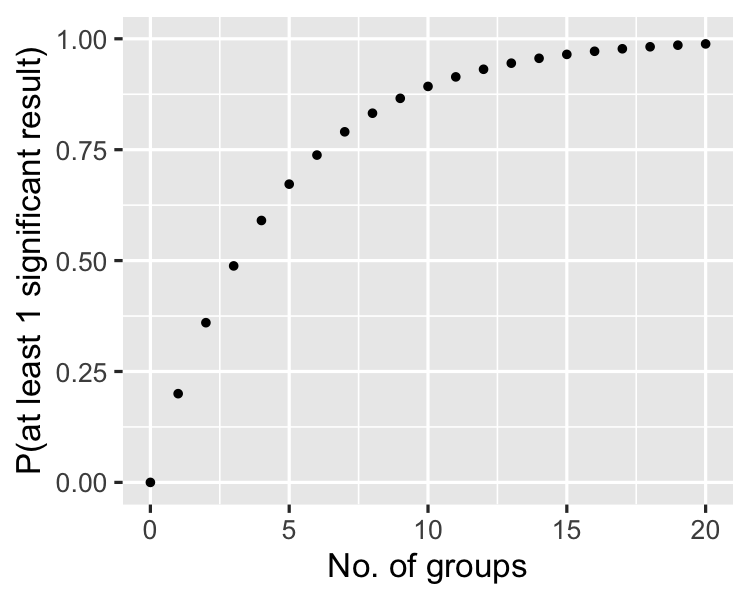
그룹 수가 증가하면...

그룹 수 대비 쌍의 수를 나타내는 산점도. 그룹 수가 증가할수록 쌍의 수가 이차적으로 증가합니다.

그룹 수 대비 유의미한 결과가 1개 이상 나올 확률을 나타내는 산점도. 그룹 수가 증가할수록 확률이 높아집니다.

본페로니 보정

pairwise.t.test(stack_overflow$converted_comp, stack_overflow$job_sat, p.adjust.method = "bonferroni")

    Pairwise comparisons using t tests with pooled SD 

data:  stack_overflow$converted_comp and stack_overflow$job_sat 

                      Very dissatisfied Slightly dissatisfied Neither Slightly satisfied
Slightly dissatisfied 1.0000            -                     -       -                 
Neither               1.0000            1.0000                -       -                 
Slightly satisfied    1.0000            1.0000                1.0000  -                 
Very satisfied        1.0000            0.0384                1.0000  0.0084            

P value adjustment method: bonferroni

유의미한 차이: "매우 만족" vs. "약간 불만족"; "매우 만족" vs. "약간 만족"

추가 방법

p.adjust.methods

"holm"  "hochberg"  "hommel"  "bonferroni"  "BH"  "BY"  "fdr"  "none"

본페로니 및 Holm 보정

p_values

0.268603 0.795778 0.295702 0.344819 0.368580 0.829315 0.003840 0.412482 0.159389 0.000838

본페로니

pmin(1, 10 * p_values)

1.00000 1.00000 1.00000 1.00000 1.00000 1.00000 0.03840 1.00000 1.00000 0.00838

Holm (대략)

pmin(1, 10:1 * sort(p_values))

0.00838 0.03456 1.00000 1.00000 1.00000 1.00000 1.00000 1.00000 1.00000 0.82931

연습해 봅시다!

R로 하는 가설 검정