가설 수립과 분포

Python으로 배우는 A/B Testing

Moe Lotfy, PhD

Principal Data Science Manager

가설 정의하기

  • 가설이란:

    • 어떤 현상을 설명하는 진술
    • 추가 조사의 출발점
    • 검증하려는 아이디어
  • 강한 가설은:

    • 검증 가능하고, 선언적이며, 간결하고, 논리적임
    • 체계적 반복을 가능하게 함
    • 일반화와 이해 확인이 쉬움
    • 실행 가능하고 집중된 제안을 도출함
Python으로 배우는 A/B Testing

가설 형식

  • 일반적 구성 형식:

    • X를 바탕으로, 우리가 Y를 하면
    • 그러면 Z가 발생한다
    • 지표 M으로 측정함
  • 대립가설 예:

    • 사용자 경험 연구를 바탕으로, 결제 페이지 디자인을 업데이트하면
    • 구매 고객 비율이 증가할 것이다
    • 구매율로 측정함
  • 귀무가설: ...구매 고객 비율은 변하지 않는다...
Python으로 배우는 A/B Testing

표본 통계량 계산

# Calculate the number of users in groups A and B
n_A = checkout[checkout['checkout_page'] == 'A']['purchased'].count()
n_B = checkout[checkout['checkout_page'] == 'B']['purchased'].count()
print('Group A users:',n_A)
print('Group B users:',n_B)
Group A users: 3000
Group B users: 3000
# Calculate the mean purchase rates of groups A and B
p_A = checkout[checkout['checkout_page'] == 'A']['purchased'].mean()
p_B = checkout[checkout['checkout_page'] == 'B']['purchased'].mean()
print('Group A mean purchase rate:',p_A)
print('Group B mean purchase rate:',p_B)
Group A mean purchase rate: 0.820
Group B mean purchase rate: 0.847
Python으로 배우는 A/B Testing

분포 시뮬레이션과 시각화

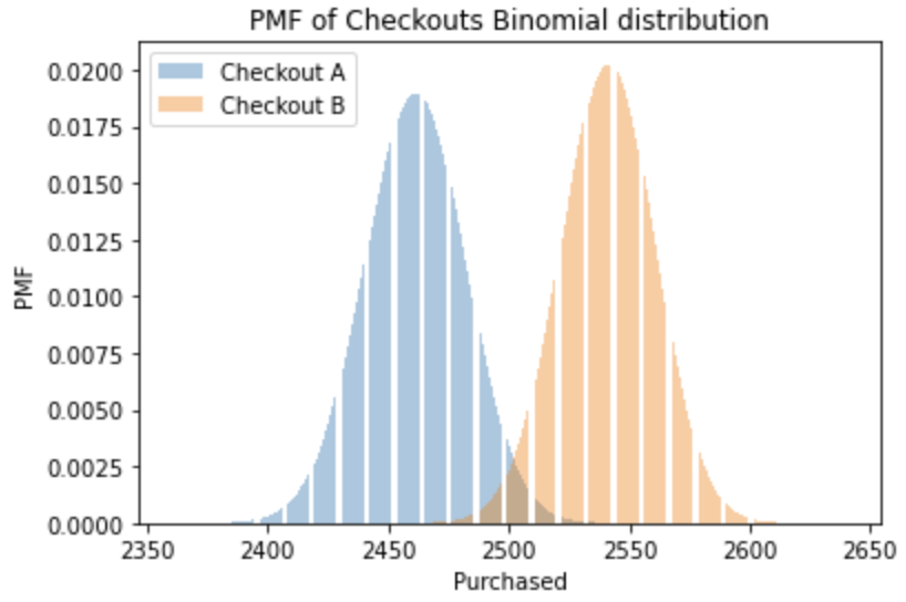
구매 확률 pn번 시행할 때 구매자 수는 이항분포를 따른다.

# Import binom from scipy library 
from scipy.stats import binom 
# Create x-axis range and Binomial distributions A and B
x = np.arange(n_A*p_A - 100, n_B*p_B + 100) 
binom_a = binom.pmf(x, n_A, p_A)
binom_b = binom.pmf(x, n_B, p_B) 
# Plot Binomial distributions A and B
plt.bar(x, binom_a, alpha=0.4, label='Checkout A')
plt.bar(x, binom_b, alpha=0.4, label='Checkout B')
plt.xlabel('Purchased')
plt.ylabel('PMF')
plt.title('PMF of Checkouts Binomial distribution')
plt.show()

결제 그룹 A와 B의 이항분포

Python으로 배우는 A/B Testing

중심극한정리

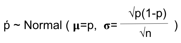
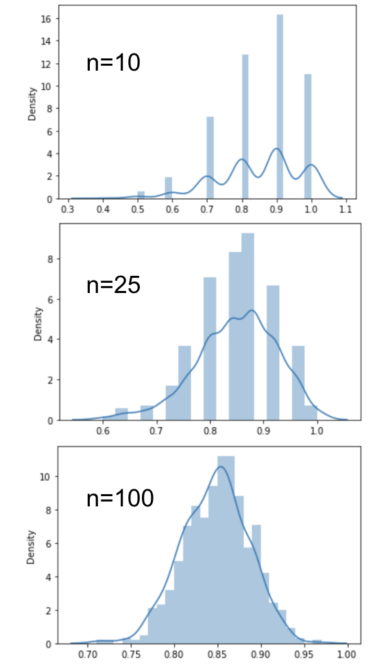
표본 크기가 충분히 크면, 표본 평균 분포 p

  • 참 모집단 평균을 중심으로 정규분포를 따름
  • 표준편차 = 평균의 표준오차
  • 원자료의 분포와 무관

비율에 대한 중심극한정리 공식

Python으로 배우는 A/B Testing

파이썬에서의 중심극한정리

# Set random seed for repeatability 
np.random.seed(47)
# Create an empty list to hold means
sampled_means = []
# Create loop to simulate 1000 sample means
for i in range(1000):
    # Take a sample of n=100
    sample = checkout['purchased'].sample(100,replace=True)
    # Get the sample mean and append to list
    sample_mean = np.mean(sample)
    sampled_means.append(sample_mean)
# Plot distribution
sns.displot(sampled_means, kde=True)
plt.show()

파이썬으로 보는 중심극한정리. 표본 크기가 커질수록 분포가 정규에 가까워짐

Python으로 배우는 A/B Testing

가설의 수학적 표현

# Import norm from scipy library 
from scipy.stats import norm
# Create x-axis range and normal distributions A and B
x = np.linspace(0.775, 0.9, 500)
norm_a = norm.pdf(x, p_A, np.sqrt(p_A*(1-p_A) / n_A))
norm_b = norm.pdf(x, p_B, np.sqrt(p_B*(1-p_B) / n_B))
# Plot normal distributions A and B
sns.lineplot(x=x, y=norm_a, ax=ax, label='Checkout A')
sns.lineplot(x=x, y=norm_b, color='orange', \
             ax=ax, label= 'Checkout B')
ax.axvline(p_A, linestyle='--')
ax.axvline(p_B, linestyle='--')
plt.xlabel('Purchased Proportion')
plt.ylabel('PDF')
plt.legend(loc="upper left")
plt.show()

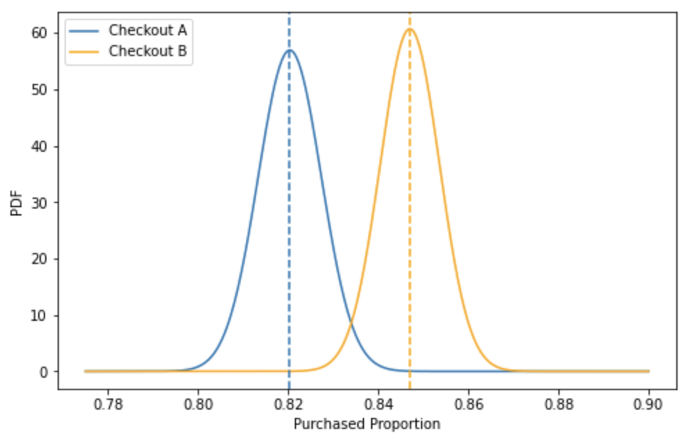
귀무가설과 대립가설의 평균 차이 플롯

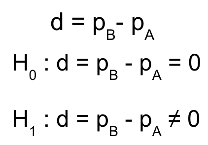
귀무가설과 대립가설의 수학적 표현

Python으로 배우는 A/B Testing

연습해 봅시다!

Python으로 배우는 A/B Testing

Preparing Video For Download...