A/B 테스트

Python으로 배우는 Bayesian 데이터 분석

Michal Oleszak

Machine Learning Engineer

A/B 테스트

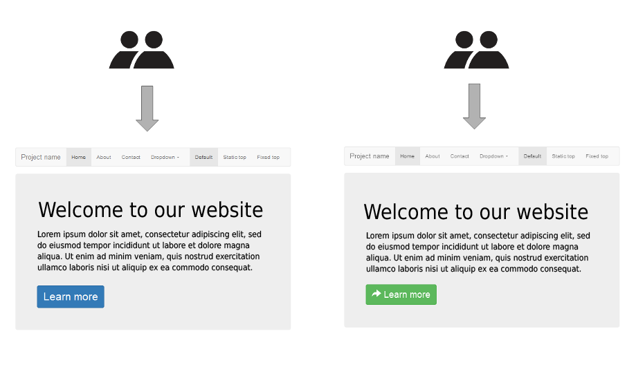
무작위 실험: 사용자를 두 그룹(A, B)으로 나눕니다

두 사용자 그룹.

¹ Picture: adapted from https://commons.wikimedia.org/wiki/File:A-B_testing_simple_example.png

A/B 테스트

무작위 실험: 사용자를 두 그룹(A, B)으로 나눕니다
각 그룹에 다른 버전을 노출합니다(예: 웹사이트 레이아웃)

두 사용자 그룹이 서로 다른 웹사이트 레이아웃을 보는 모습.

¹ Picture: adapted from https://commons.wikimedia.org/wiki/File:A-B_testing_simple_example.png

A/B 테스트

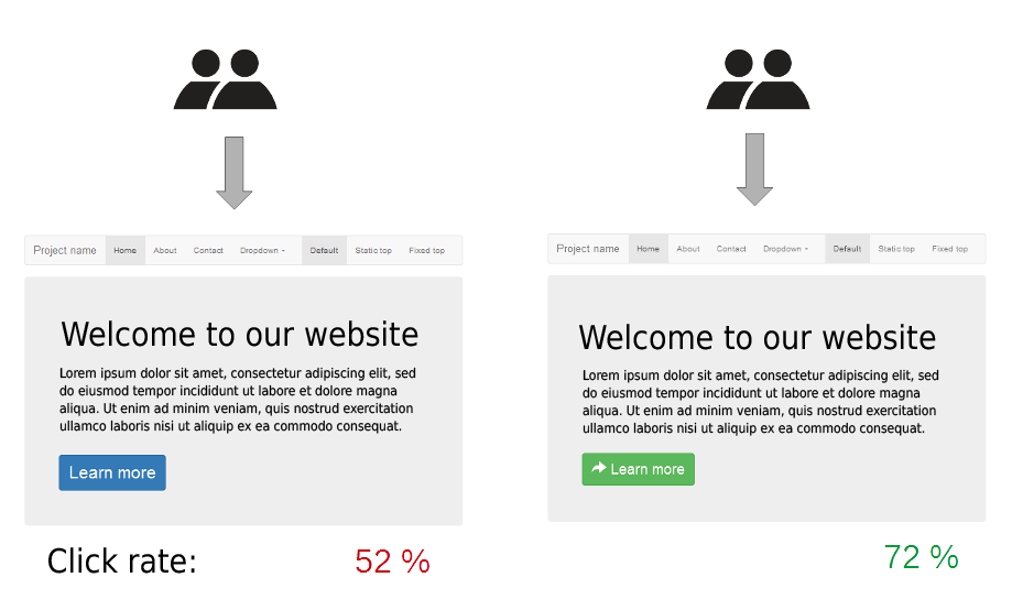
무작위 실험: 사용자를 두 그룹(A, B)으로 나눕니다
각 그룹에 다른 버전을 노출합니다(예: 웹사이트 레이아웃)
특정 지표(예: 클릭률)로 어느 그룹이 더 높은지 비교합니다

두 사용자 그룹이 서로 다른 웹사이트 레이아웃을 보며, 한쪽이 더 높은 클릭률을 보임.

¹ Picture: adapted from https://commons.wikimedia.org/wiki/File:A-B_testing_simple_example.png

A/B 테스트: 빈도주의 접근

가설 검정 기반
A와 B의 성능이 같은지 확인
A가 B보다 얼마나 나은지는 말해주지 않음

A/B 테스트: 베이지안 접근

웹사이트 레이아웃 A, B의 사후 클릭률을 계산해 비교합니다
A가 B보다 나을 확률을 직접 계산합니다
얼마나 더 나은지도 정량화합니다
오결정 시 기대 손실을 추정합니다

A/B 테스트: 베이지안 접근

사용자가 웹사이트에 오면 두 경우:
- 클릭(성공)
- 클릭 없음(실패)
이항분포 사용! (성공확률 = 클릭률)

베타 사후분포 시뮬레이션

사전분포가 $Beta(a, b)$이면, 사후분포는 $Beta(x, y)$이며:

$x = \text{NumberOfSuccesses} + a$

$y = \text{NumberOfObservations} - \text{NumberOfSuccesses} + b$

def simulate_beta_posterior(trials, beta_prior_a, beta_prior_b):
    num_successes = np.sum(trials)
    posterior_draws = np.random.beta(
      num_successes + beta_prior_a, 
      len(trials) - num_successes + beta_prior_b, 
      10000
    )
    return posterior_draws

사후분포 비교

1(클릭)과 0(미클릭) 리스트:

print(A_clicks)
print(B_clicks)

[0 1 1 0 0 0 0 0 0 0 1 ... ]
[0 0 0 1 0 0 0 1 1 0 1 ... ]

각 레이아웃의 사후표본 시뮬레이션:

A_posterior = simulate_beta_posterior(A_clicks, 1, 1)
B_posterior = simulate_beta_posterior(B_clicks, 1, 1)

사후분포 그리기:

sns.kdeplot(A_posterior, shade=True, label="A")
sns.kdeplot(B_posterior, shade=True, label="B")
plt.show()

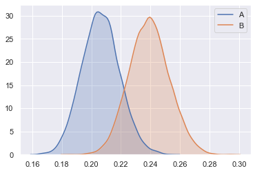
부분적으로 겹치는 두 사후분포 밀도 그래프.

사후분포 비교

B와 A의 사후 차이:

diff = B_posterior - A_posterior

sns.kdeplot(diff, shade=True, label="difference: A-B")
plt.show()

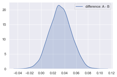
거의 모든 확률질량이 0 위에 있는 밀도 그래프.

B가 더 나을 확률:

(diff > 0).mean()

0.9639

기대 손실

열등한 버전을 배포하면 클릭을 얼마나 잃을까요?

# A가 더 좋을 때의 차이(B-A)
loss = diff[diff < 0]


# 기대(평균) 손실
expected_loss = loss.mean()
print(expected_loss)

-0.0077850237030215215

광고 데이터

print(ads)

                               user_id   product site_version                 time  banner_clicked
0     f500b9f27ac611426935de6f7a52b71f   clothes      desktop  2019-01-28 16:47:08               0
1     cb4347c030a063c63a555a354984562f  sneakers       mobile  2019-03-31 17:34:59               0
2     89cec38a654319548af585f4c1c76b51   clothes       mobile  2019-02-06 09:22:50               0
3     1d4ea406d45686bdbb49476576a1a985  sneakers       mobile  2019-05-23 08:07:07               0
4     d14b9468a1f9a405fa801a64920367fe   clothes       mobile  2019-01-28 08:16:37               0
...                                ...       ...          ...                  ...             ...
9995  7ca28ccde263a675d7ab7060e9ed0eca   clothes       mobile  2019-02-02 08:19:39               0
9996  7e2ec2631332c6c4527a1b78c7ede789   clothes       mobile  2019-04-04 03:27:05               0
9997  3b828da744e5785f1e67b5df3fda5571   clothes       mobile  2019-04-15 15:59:06               0
9998  6cce0527245bcc8519d698af2224c04a   clothes       mobile  2019-05-21 20:43:21               0
9999  8cf87a02f96327a1a8a93814f34d0d0c  sneakers       mobile  2019-03-02 21:27:57               0

A/B 테스트를 해봅시다!

Python으로 배우는 Bayesian 데이터 분석