백색잡음
R로 배우는 시계열 예측

Rob J. Hyndman
Professor of Statistics at Monash University
백색잡음
set.seed(3)          # Reproducibility
wn <- ts(rnorm(36))  # White noise
autoplot(wn)         # Plot!
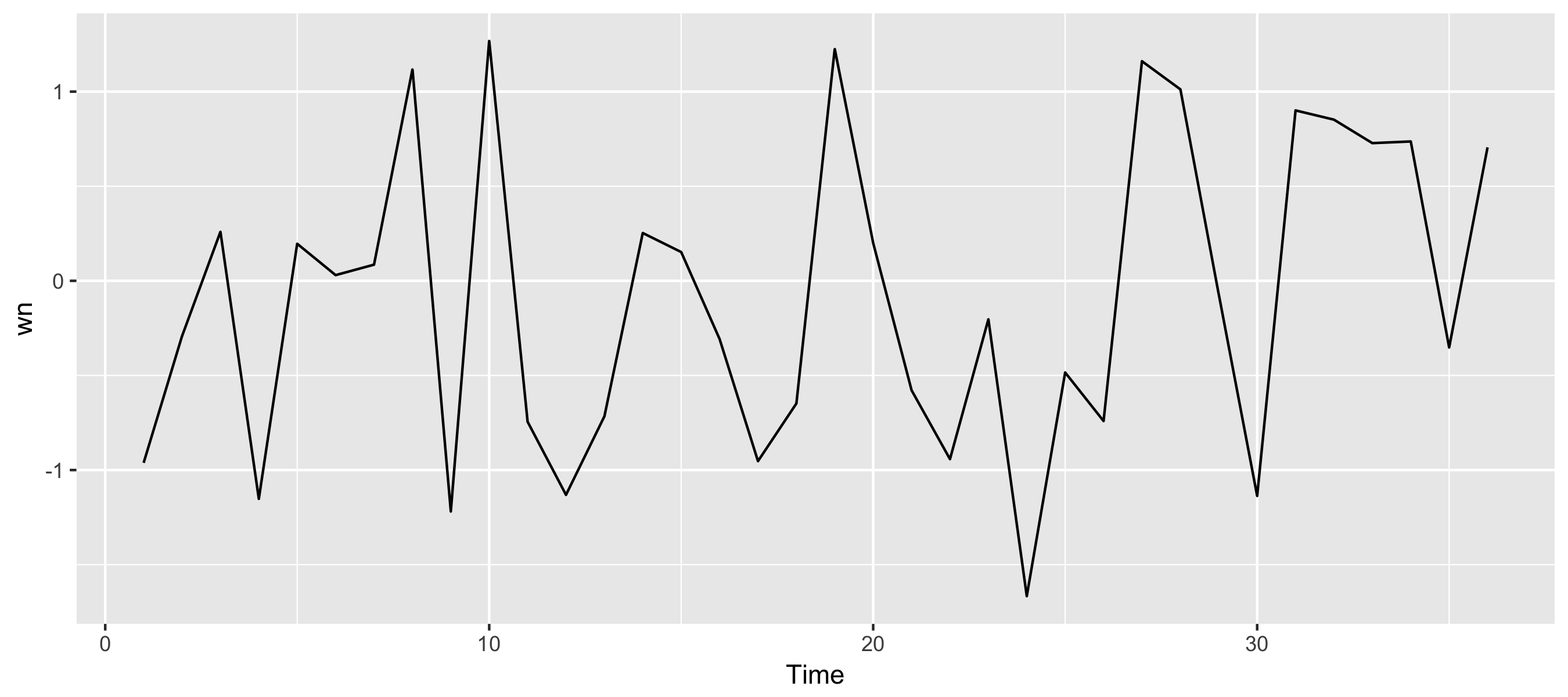
"백색잡음"은 iid 자료의 시계열입니다
백색잡음 ACF
ggAcf(wn) +
    ggtitle("Sample ACF for white noise")
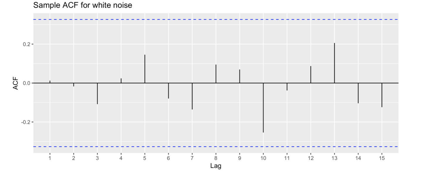
백색잡음 ACF
ggAcf(wn) +
    ggtitle("Sample ACF for white noise")
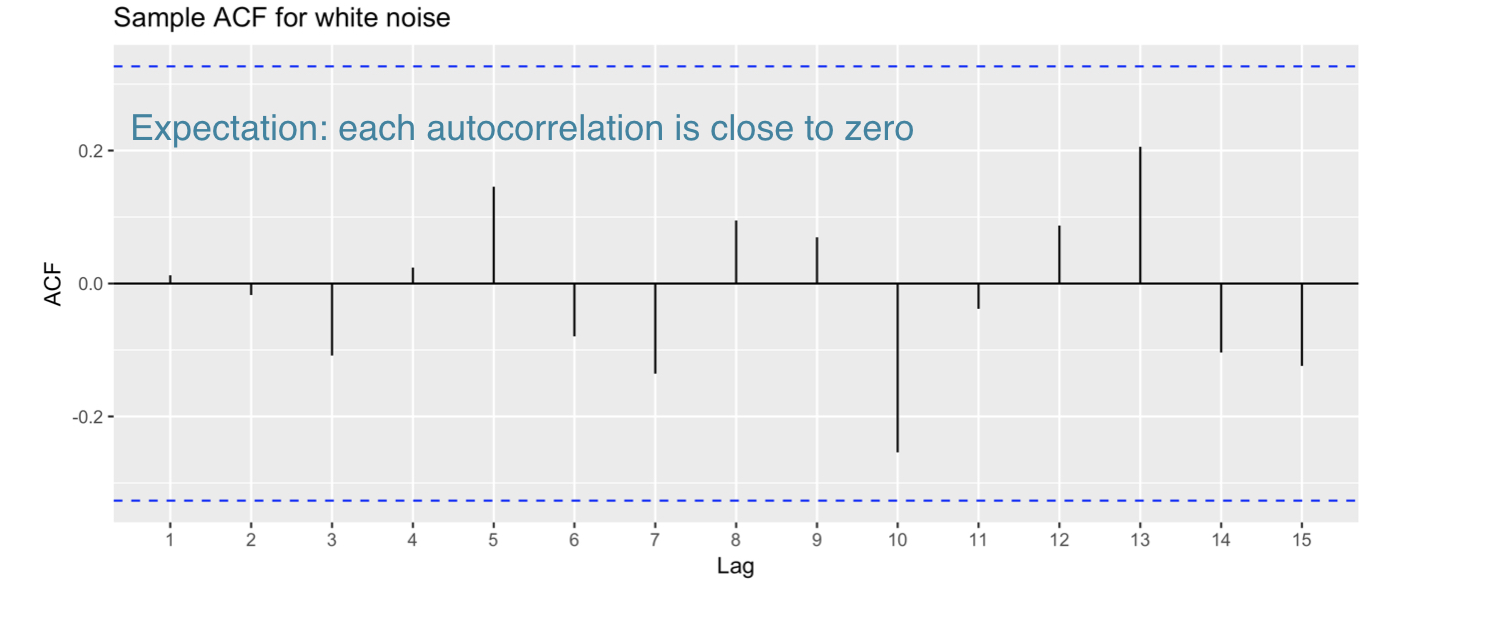
백색잡음 ACF
ggAcf(wn) +
    ggtitle("Sample ACF for white noise")
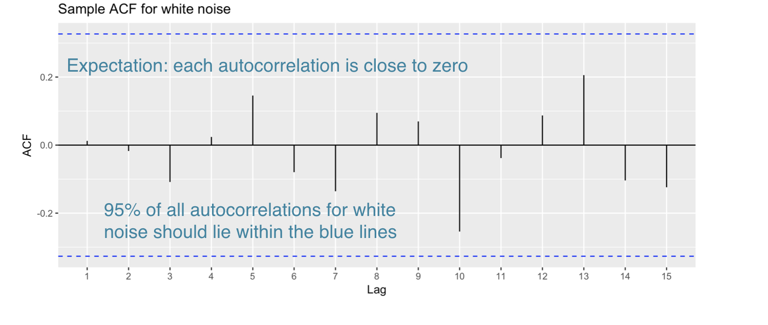
백색잡음 ACF
ggAcf(wn) +
    ggtitle("Sample ACF for white noise")
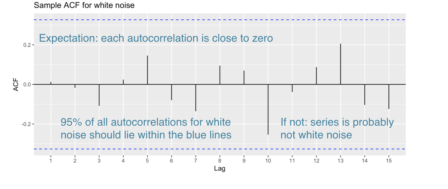
예시: 돼지 도축
pigs <- window(pigs, start=1990)
autoplot(pigs/1000) +
  xlab("Year") +
  ylab("thousands") +
  ggtitle("Monthly number of pigs slaughtered in Victoria")
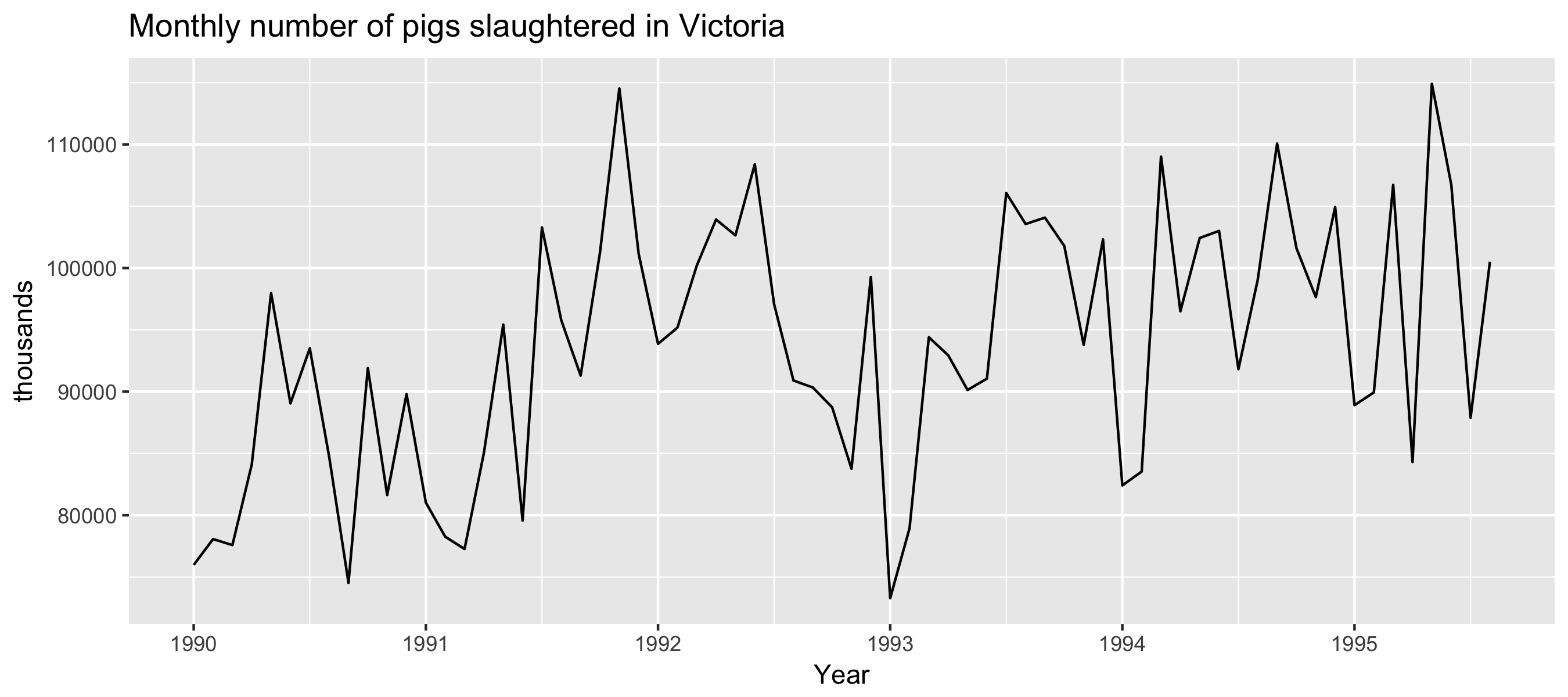
예시: 돼지 도축
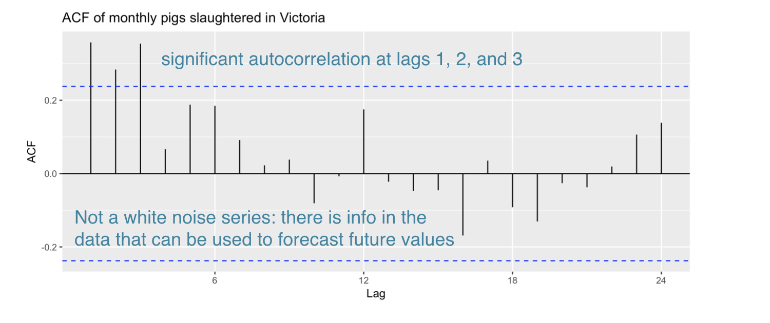
ggAcf(pigs) +
  ggtitle("ACF of monthly pigs slaughtered
          in Victoria")
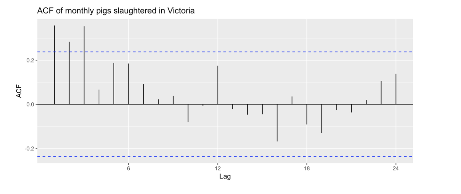
예시: 돼지 도축
ggAcf(pigs) +
  ggtitle("ACF of monthly pigs slaughtered
          in Victoria")
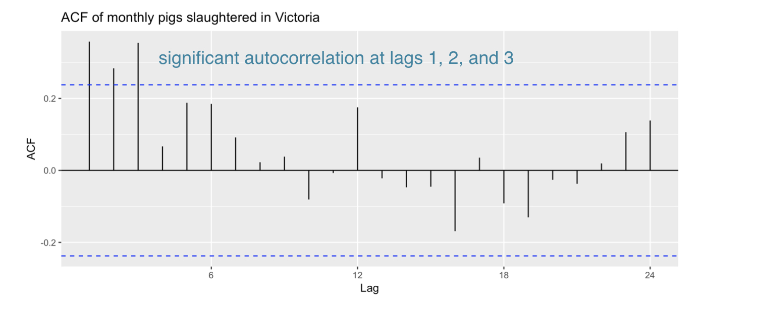
예시: 돼지 도축
ggAcf(pigs) +
  ggtitle("ACF of monthly pigs slaughtered
          in Victoria")