계절 ARIMA 모델

R로 배우는 시계열 예측

Rob J. Hyndman

Professor of Statistics at Monash University

ARIMA 모델

ch4_vid3_slides.003.png

d = 시차 1 차분 횟수
p = 일반 AR 시차 개수:
q = 일반 MA 시차 개수:

ARIMA 모델

ch4_vid3_slides.007.png

d = 시차 1 차분 횟수
p = 일반 AR 시차 개수:
q = 일반 MA 시차 개수:

ARIMA 모델

ch4_vid3_slides.008.png

d = 시차 1 차분 횟수
p = 일반 AR 시차 개수: $\ y_{t-1}, y_{t-2},...,y_{t-p}$
q = 일반 MA 시차 개수: $\ \epsilon_{t-1}, \epsilon_{t-2},...,\epsilon_{t-q}$
D = 계절 차분 횟수
P = 계절 AR 시차 개수: $\ y_{t-m}, y_{t-2m},...,y_{t-Pm}$
Q = 계절 MA 시차 개수:$\ \epsilon_{t-m}, \epsilon_{t-2m},...,\epsilon_{t-Qm}$
m = 연간 관측치 수

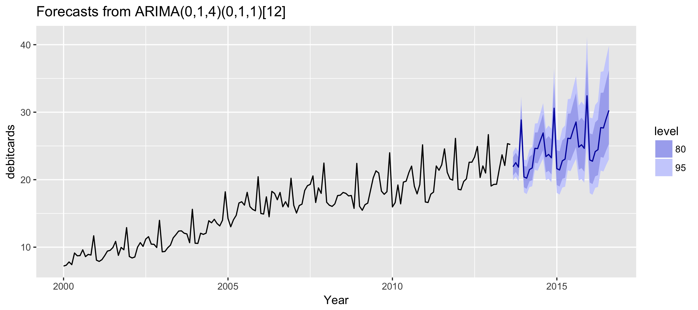
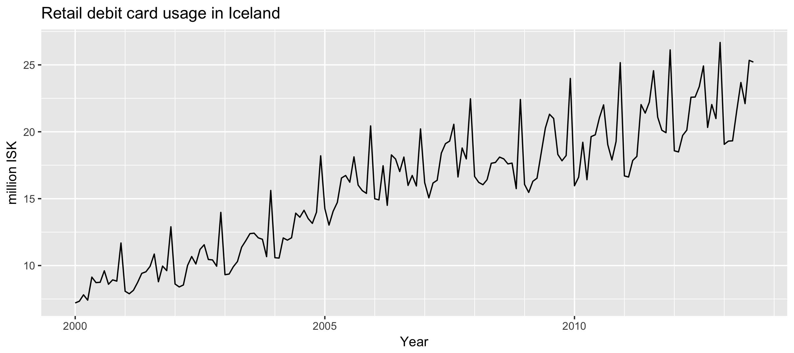
예시: 아이슬란드 월별 소매 직불카드 사용

autoplot(debitcards) +
  xlab("Year") + ylab("million ISK") +
  ggtitle("Retail debit card usage in Iceland")

예시: 아이슬란드 월별 소매 직불카드 사용

fit <- auto.arima(debitcards, lambda = 0)
fit

Series: debitcards
ARIMA(0,1,4)(0,1,1)[12]
Box Cox transformation: lambda= 0
Coefficients:
         ma1    ma2    ma3     ma4    sma1
      -0.796  0.086  0.263  -0.175  -0.814
s.e.   0.082  0.099  0.100   0.080   0.112
sigma^2 estimated as 0.00232:  log likelihood=239.3
AIC=-466.7   AICc=-466.1   BIC=-448.6

예시: 아이슬란드 월별 소매 직불카드 사용

fit %>%
  forecast(h = 36) %>%
  autoplot() + xlab("Year")

Lass uns üben!

R로 배우는 시계열 예측