R에서 tidymodels로 모델링하기
David Svancer
Data Scientist
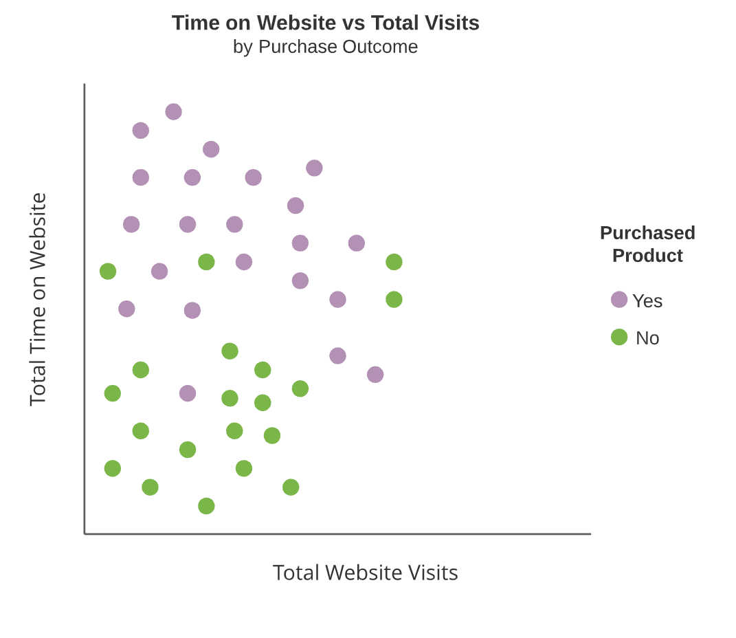
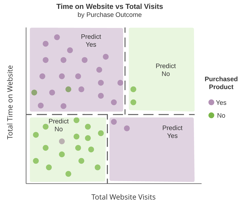
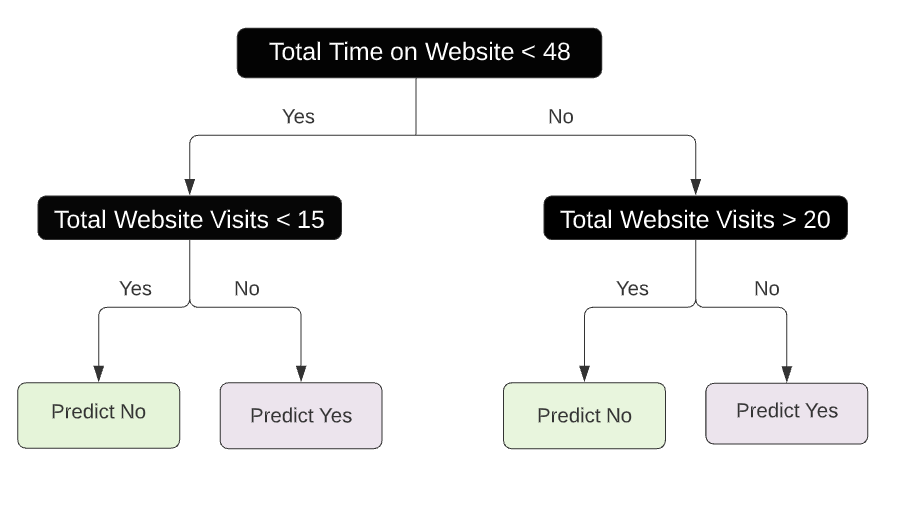
의사결정나무는 예측자 공간을 직사각형 구역으로 분할합니다
재귀적 이진 분할

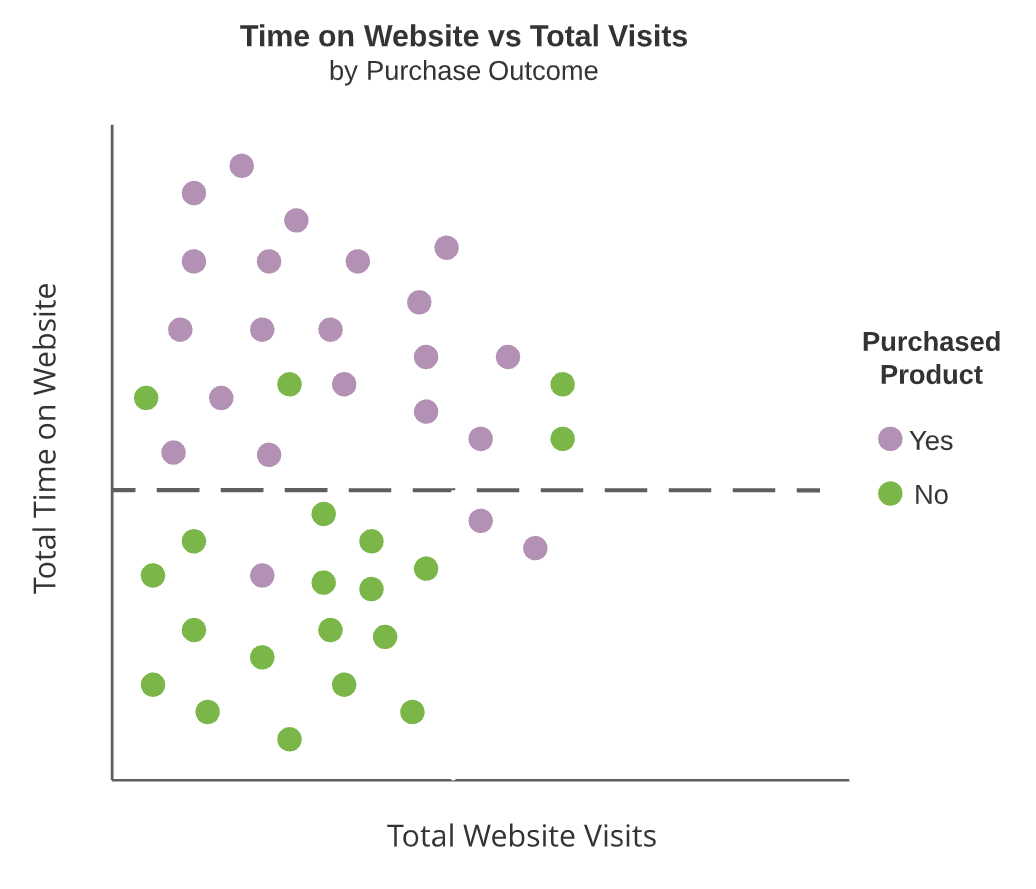
의사결정나무는 예측자 공간을 직사각형 구역으로 분할합니다
재귀적 이진 분할

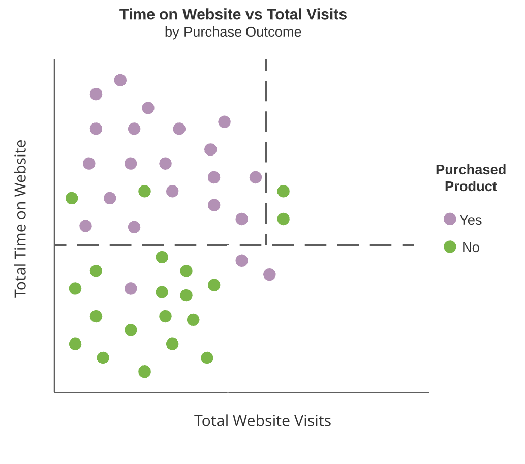
의사결정나무는 예측자 공간을 직사각형 구역으로 분할합니다
재귀적 이진 분할

의사결정나무는 예측자 공간을 직사각형 구역으로 분할합니다
재귀적 이진 분할

의사결정나무는 예측자 공간을 직사각형 구역으로 분할합니다
재귀적 이진 분할
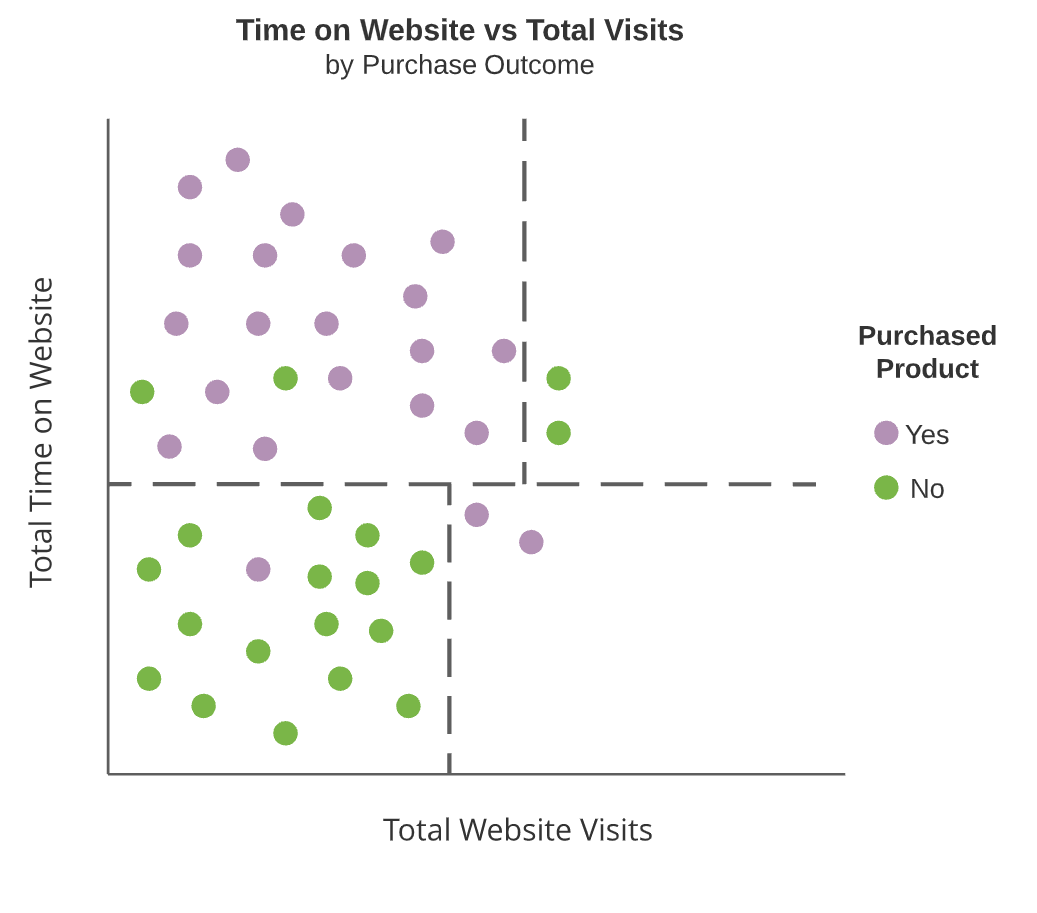
뚜렷한 직사각형 구역 생성


내부 노드는 점선, 단말 노드는 강조된 직사각형 구역입니다

parsnip에서의 모델 명세
decision_tree()parsnip의 의사결정나무 일반 인터페이스'rpart''classification' 또는 'regression''classification' 필요dt_model <- decision_tree() %>%set_engine('rpart') %>%set_mode('classification')
리드 스코어링 데이터 변환
recipe 객체에 인코딩관리할 두 개의 R 객체
parsnip 모델과 recipe 명세leads_recipe <- recipe(purchased ~ ., data = leads_training) %>%step_corr(all_numeric(), threshold = 0.9) %>% step_normalize(all_numeric()) %>% step_dummy(all_nominal(), -all_outcomes())
leads_recipe
Data Recipe
Inputs:
role #variables
outcome 1
predictor 6
Operations:
Correlation filter on all_numeric()
Centering and scaling for all_numeric()
Dummy variables from all_nominal(), -all_outcomes()
workflows 패키지는 모델 과정을 간소화합니다
parsnip 모델과 recipe 객체를 하나의 workflow 객체로 결합
workflow() 함수로 초기화
add_model()로 모델 추가add_recipe()로 recipe 추가recipe가 아닌 명세여야 함leads_wkfl <- workflow() %>%add_model(dt_model) %>%add_recipe(leads_recipe)leads_wkfl
== Workflow =====================
Preprocessor: Recipe
Model: decision_tree()
-- Preprocessor -----------------
3 Recipe Steps
* step_corr()
* step_normalize()
* step_dummy()
-- Model --------------------------
Decision Tree Model Specification (classification)
Computational engine: rpart
workflow 객체 학습
workflow를 last_fit()에 전달하고 데이터 분할 객체 제공collect_metrics()로 평가 결과 확인내부 동작
recipe 학습 및 적용leads_wkfl_fit <- leads_wkfl %>% last_fit(split = leads_split)leads_wkfl_fit %>% collect_metrics()
# A tibble: 2 x 3
.metric .estimator .estimate
<chr> <chr> <dbl>
1 accuracy binary 0.771
2 roc_auc binary 0.775
last_fit()으로 학습된 workflow는 collect_predictions()에 전달할 수 있습니다
yardstick 함수로 사용자 정의 성능 지표 탐색 가능leads_wkfl_preds <- leads_wkfl_fit %>% collect_predictions()leads_wkfl_preds
# A tibble: 332 x 6
id .pred_yes .pred_no .row .pred_class purchased
<chr> <dbl> <dbl> <int> <fct> <fct>
train/test split 0.120 0.880 2 no no
train/test split 0.755 0.245 17 yes yes
train/test split 0.120 0.880 21 no no
train/test split 0.120 0.880 22 no no
train/test split 0.755 0.245 24 yes yes
# ... with 327 more rows
metric_set()으로 사용자 정의 지표 집합 생성
예측 데이터셋을 leads_metrics()에 전달해 지표 계산
leads_metrics <- metric_set(roc_auc, sens, spec)leads_wkfl_preds %>% leads_metrics(truth = purchased, estimate = .pred_class, .pred_yes)
# A tibble: 3 x 3
.metric .estimator .estimate
<chr> <chr> <dbl>
1 sens binary 0.75
2 spec binary 0.783
3 roc_auc binary 0.775
은행의 소매 대출 금융 데이터
loan_default
loans_df
# A tibble: 872 x 8
loan_default loan_purpose missed_payment_2_yr loan_amount interest_rate installment annual_income debt_to_income
<fct> <fct> <fct> <int> <dbl> <dbl> <dbl> <dbl>
no debt_consolidation no 25000 5.47 855. 62823 39.4
yes medical no 10000 10.2 364. 40000 24.1
no small_business no 13000 6.22 442. 65000 14.0
no small_business no 36000 5.97 1152. 125000 8.09
yes small_business yes 12000 11.8 308. 65000 20.1
# ... with 867 more rows
R에서 tidymodels로 모델링하기