분류 모델
R에서 tidymodels로 모델링하기

David Svancer
Data Scientist
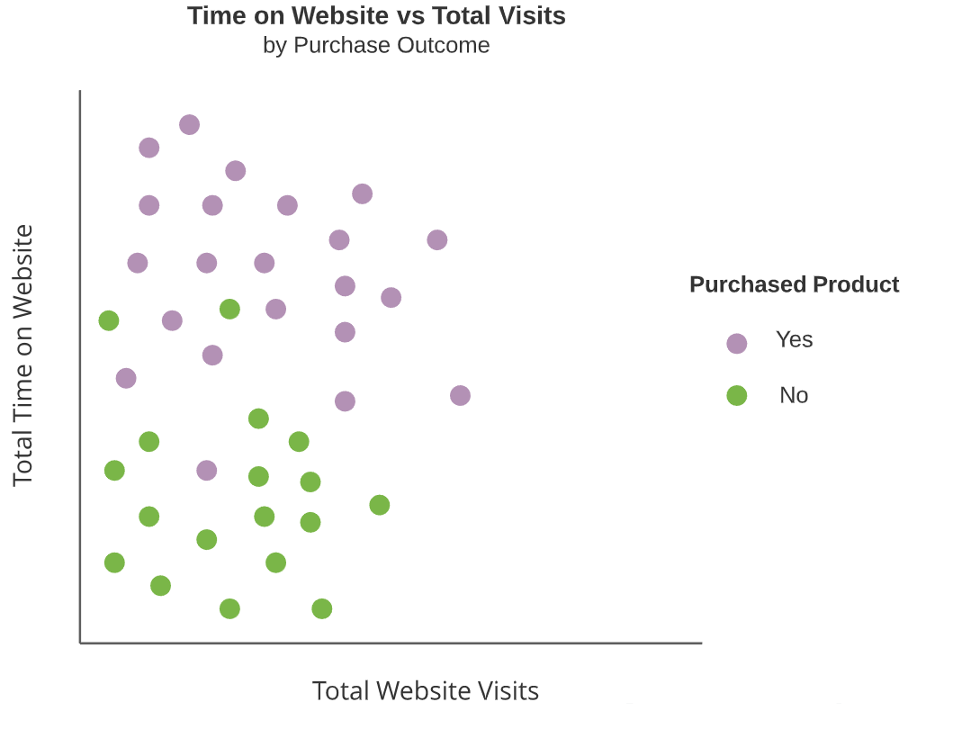
제품 구매 예측
분류 모델은 범주형 결과 변수를 예측합니다
- 제품 구매 예측
| purchased | total_time | total_visits |
|---|---|---|
| yes | 800 | 3 |
| yes | 978 | 7 |
| no | 220 | 4 |
| no | 124 | 5 |
| yes | 641 | 4 |
분류 알고리즘
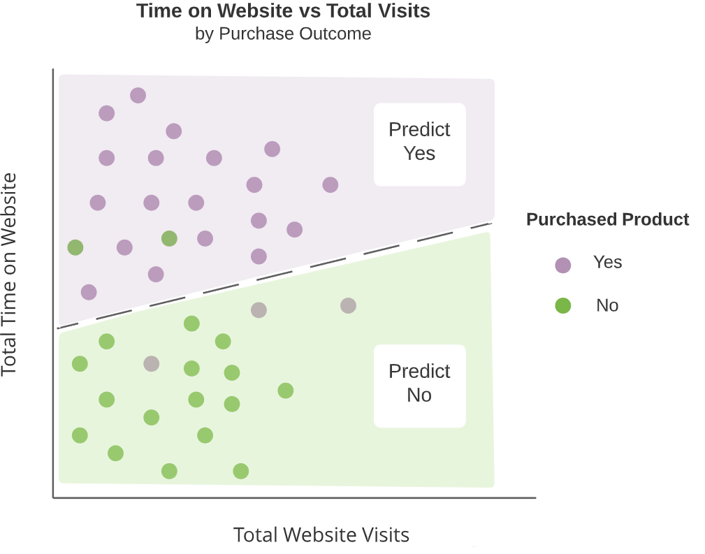
목표: 예측 변수 값 공간을 겹치지 않는 구역으로 나눕니다
- 각 구역에서 동일한 범주형 결과를 예측
분류 알고리즘
목표: 예측 변수 값 공간을 겹치지 않는 구역으로 나눕니다
- 각 구역에서 동일한 범주형 결과를 예측
로지스틱 회귀
- 결과 범주 간에 선형 경계를 만드는 대표 분류 알고리즘
리드 스코어링 데이터
leads_df
# A tibble: 1,328 x 7
   purchased total_visits total_time pages_per_visit total_clicks lead_source    us_location
   <fct>            <dbl>      <dbl>           <dbl>        <dbl> <fct>          <fct>
 1 yes                  7       1148            7              59 direct_traffic west
 2 no                   8        100            2.67           24 direct_traffic west
 3 no                   5        228            2.5            25 email          southeast
 4 no                   7        481            2.33           21 organic_search west
 5 no                   4        177            4              37 direct_traffic west
 6 no                   2       1273            2              26 email          midwest
 7 no                   3        711            3              28 organic_search west
 8 no                   3        166            3              32 direct_traffic southeast
 9 no                   3          7            3              23 organic_search west
10 no                   6        562            6              48 organic_search southeast
# ... with 1,318 more rows
데이터 리샘플링
모델 적합의 첫 단계
initial_split()로 데이터 분할 객체 생성training(),testing()으로 학습/테스트 세트 생성
leads_split <- initial_split(leads_df, prop = 0.75, strata = purchased)leads_training <- leads_split %>% training()leads_test <- leads_split %>% testing()
로지스틱 회귀 모델 명세
parsnip의 모델 명세
logistic_reg()parsnip의 로지스틱 회귀용 일반 인터페이스- 일반 엔진: 'glm'
- 모드: 'classification'
logistic_model <- logistic_reg() %>%set_engine('glm') %>%set_mode('classification')
모델 학습
모델을 명세한 후 fit()으로 학습
- 모델 객체를
fit()에 전달 - 모델 수식 지정
- 학습 데이터는
data로 제공
logistic_fit <- logistic_model %>%fit(purchased ~ total_visits + total_time,data = leads_training)
결과 범주 예측
predict() 함수
new_data는 예측할 데이터셋 지정type'class'는 범주 예측 제공
predict()의 표준 출력
- tibble 반환
type이'class'이면.pred_class라는 팩터 열 반환
class_preds <- logistic_fit %>%predict(new_data = leads_test,type = 'class')class_preds
# A tibble: 332 x 1
   .pred_class
   <fct>
 1 no
 2 yes
 3 no
 4 no
 5 yes
 # ... with 327 more rows
추정 확률
type을 'prob'로 설정하면 각 결과 범주의 추정 확률을 제공합니다
predict()는 여러 열이 있는 tibble을 반환합니다
- 결과 범주마다 한 열
- 열 이름 규칙:
.pred_{outcome_category}
prob_preds <- logistic_fit %>%
  predict(new_data = leads_test,
          type = 'prob')

prob_preds
# A tibble: 332 x 2
   .pred_yes .pred_no
       <dbl>    <dbl>
 1    0.134     0.866
 2    0.729     0.271
 3    0.133     0.867
 4    0.0916    0.908
 5    0.598     0.402
# ... with 327 more rows
결과 결합
yardstick 패키지로 평가하려면 결과 tibble이 필요합니다
테스트셋의 정답과 예측 tibble은 bind_cols()로 결합할 수 있습니다
leads_results <- leads_test %>%
  select(purchased) %>%
  bind_cols(class_preds, prob_preds)
leads_results
# A tibble: 332 x 4
   purchased .pred_class .pred_yes .pred_no
   <fct>     <fct>           <dbl>    <dbl>
 1 no        no             0.134     0.866
 2 yes       yes            0.729     0.271
 3 no        no             0.133     0.867
 4 no        no             0.0916    0.908
 5 yes       yes            0.598     0.402
# ... with 327 more rows
통신 데이터
telecom_df
# A tibble: 975 x 9
   canceled_service cellular_service avg_data_gb avg_call_mins avg_intl_mins internet_service   contract    months_with_company monthly_charges
   <fct>            <fct>               <dbl>         <dbl>        <dbl>         <fct>           <fct>               <dbl>           <dbl>
 1 yes              single_line         7.78           497         127         fiber_optic     month_to_month         7              76.4
 2 yes              single_line         9.04           336         88          fiber_optic     month_to_month         10             94.9
 3 no               single_line         10.3           262         55          fiber_optic     one_year               50             103.
 4 yes              multiple_lines      5.08           250         107         digital         one_year               53             60.0
 5 no               multiple_lines      8.05           328         122         digital         two_year               50             75.2
 6 no               single_line         9.3            326         114         fiber_optic     month_to_month         25             95.7
 7 yes              multiple_lines      8.01           525         97          fiber_optic     month_to_month         19             83.6
 8 no               multiple_lines      9.4            312         147         fiber_optic     one_year               50             99.4
 9 yes              single_line         5.29           417         96          digital         month_to_month         8              49.8
10 no               multiple_lines      9.96           340         136         fiber_optic     month_to_month         61             106.
# ... with 965 more rows
연습해 봅시다!
R에서 tidymodels로 모델링하기

