축하합니다!

R에서 결측치 다루기

Nicholas Tierney

Statistician

챕터 1

결측값이란

결측값은 기록되어야 했지만 기록되지 않은 값입니다.

결측값 요약하기

miss_var_summary(airquality)

A tibble: 6 x 3
  variable n_miss pct_miss 
  <chr>     <int>    <dbl> 
1 Ozone        37    24.2  
2 Solar.R       7     4.58 
3 Wind          0     0    
4 Temp          0     0    
5 Month         0     0    
6 Day           0     0

챕터 1

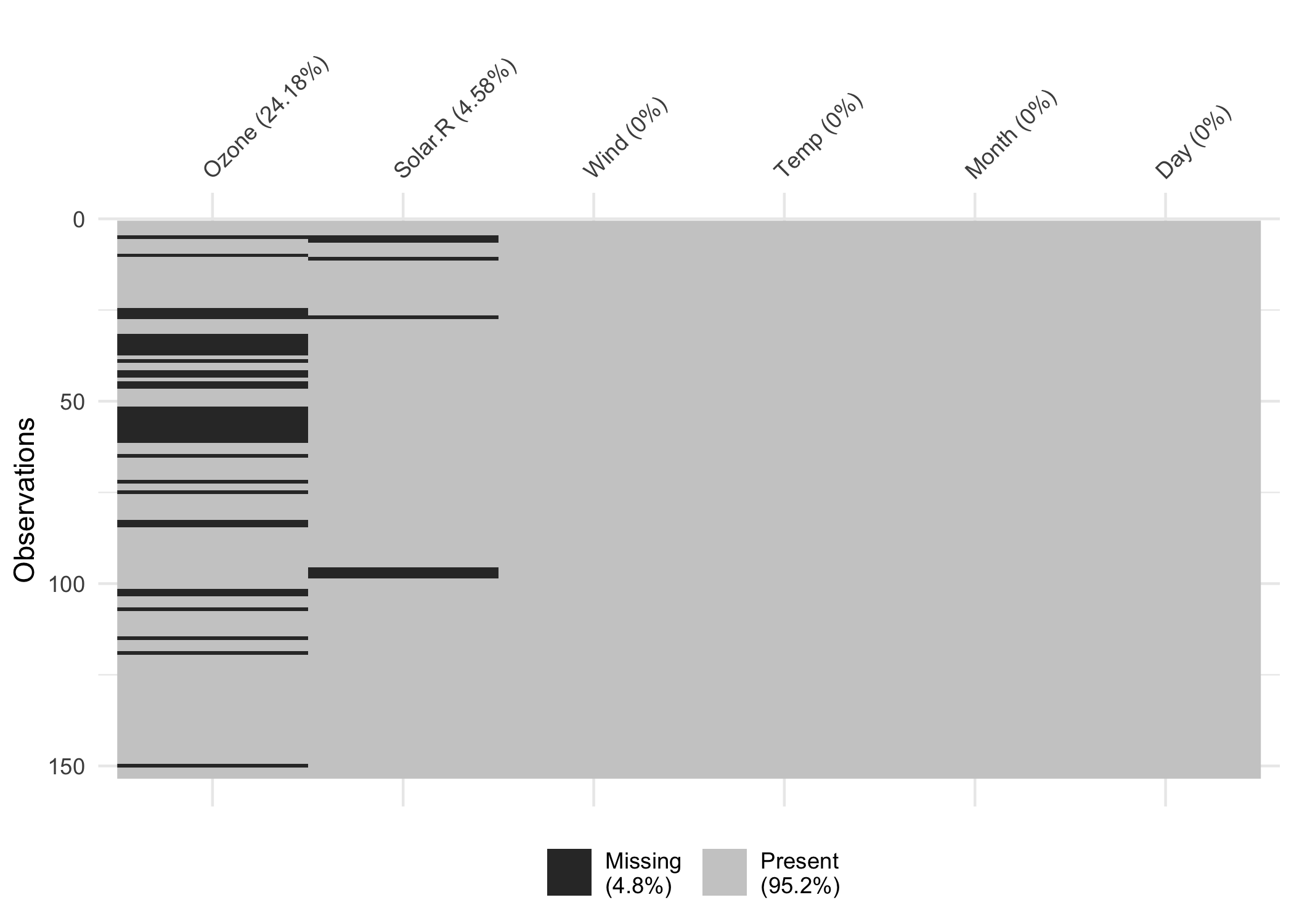
vis_miss(airquality)

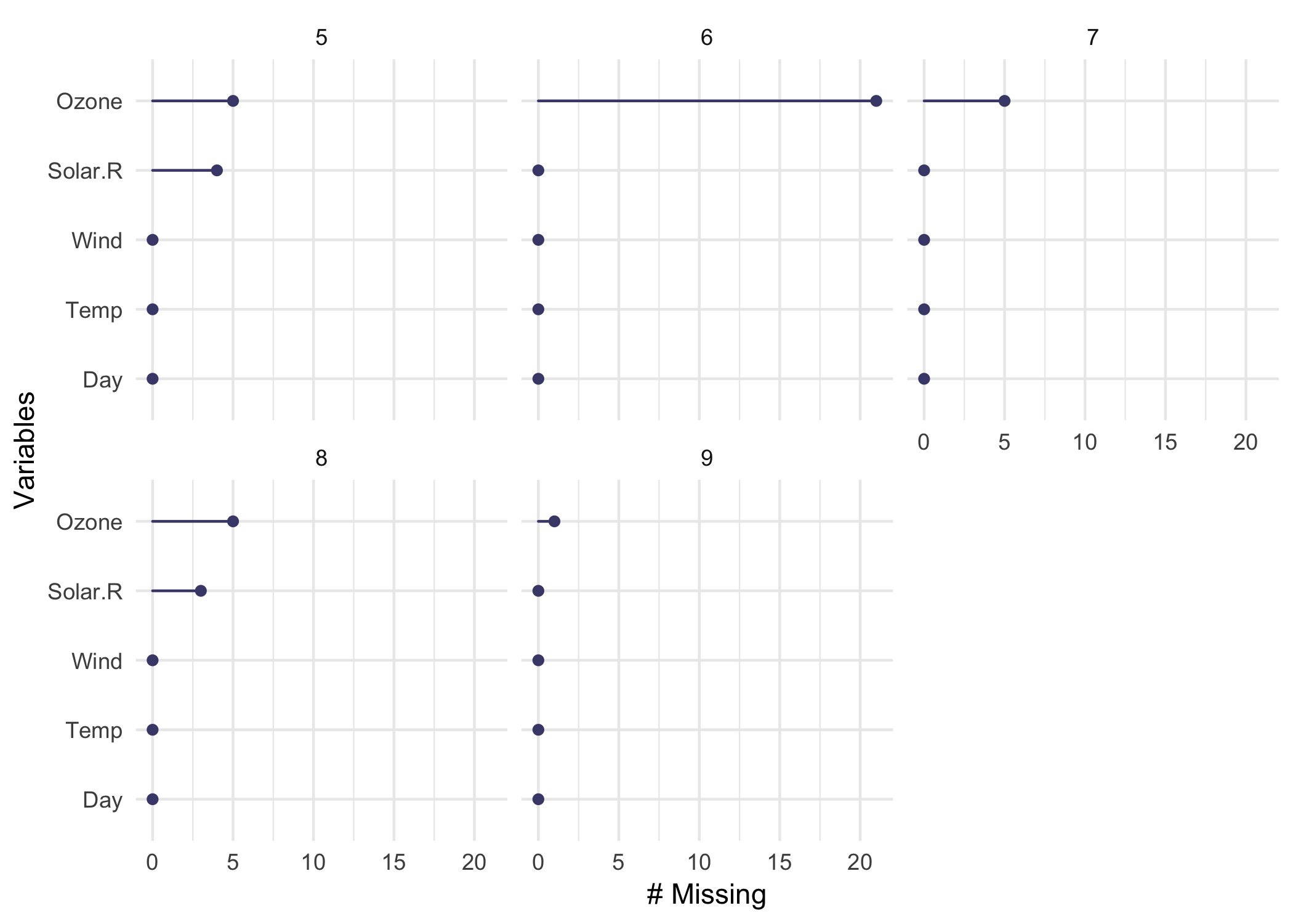
gg_miss_var(airquality, facet=Month)

챕터 2

대체 결측값 찾기

miss_scan_count(data = pacman, 
                search = list("N/A"))

대체 결측값 바꾸기

replace_with_na(pacman, 
                replace = list(
                  year = c("N/A"),
                  score = c("N/A")))

암묵적 결측값

frogger_tidy <- frogger %>% 
  complete(time, name)

결측 데이터 의존성

MCAR
MAR
MNAR

챕터 3

섀도 매트릭스, 나뷸러 데이터

nabular(airquality)

 # A tibble: 153 x 12
    Ozone Solar.R  Wind  Temp 
    <int>   <int> <dbl> <int> 
  1   41     190   7.4    67  
  2   36     118   8      72  
  3   12     149  12.6    74  
 # ... with 150 more rows, and 3 
 # more variables: Month <int>, Day <int>,
 # Ozone_NA <fct>, Solar.R_NA <fct>, 
 # Wind_NA <fct>, Temp_NA <fct>,
 # Month_NA <fct>, Day_NA <fct>

결측 탐색, 요약을 값과 연결

oceanbuoys %>%
  bind_shadow() %>%
  group_by(humidity_NA) %>%
  summarize(
    wind_ew_mean = mean(wind_ew))

 # A tibble: 2 x 2
   humidity_NA wind_ew_mean
   <fct>              <dbl>
 1 !NA                -3.78
 2 NA                 -3.30

챕터 3

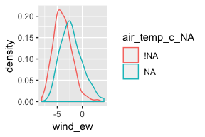
결측에 따라 값이 어떻게 달라지는가

nabular(oceanbuoys) %>%
  ggplot(aes(x = wind_ew, 
             color = air_temp_c_NA)) + 
  geom_density()

공기 온도별 ggplot 밀도

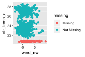
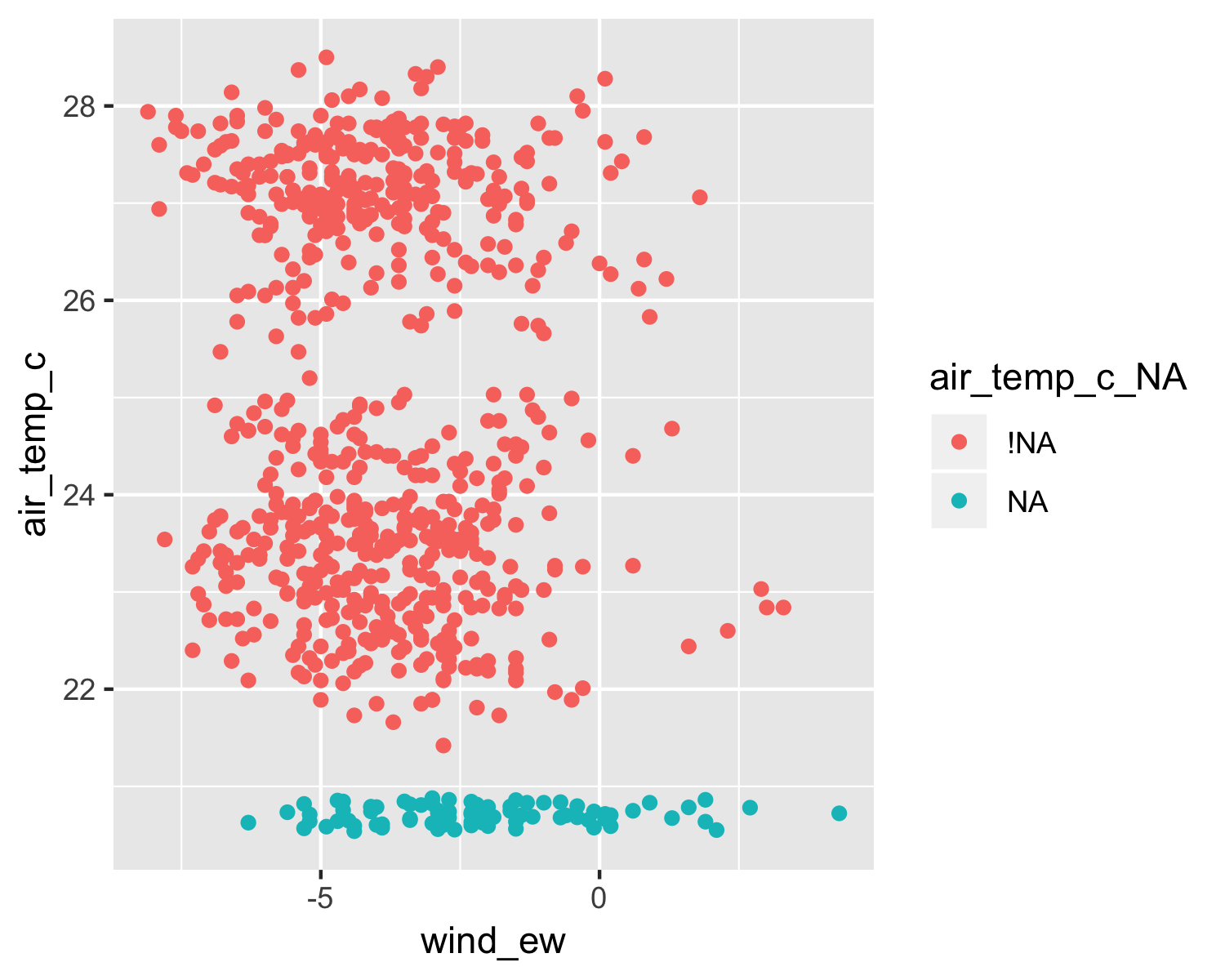
두 변수에서 결측 시각화

ggplot(oceanbuoys,
       aes(x = wind_ew,
           y = air_temp_c)) + 
  geom_miss_point()

gg-miss-point

챕터 4

좋은/나쁜 대치

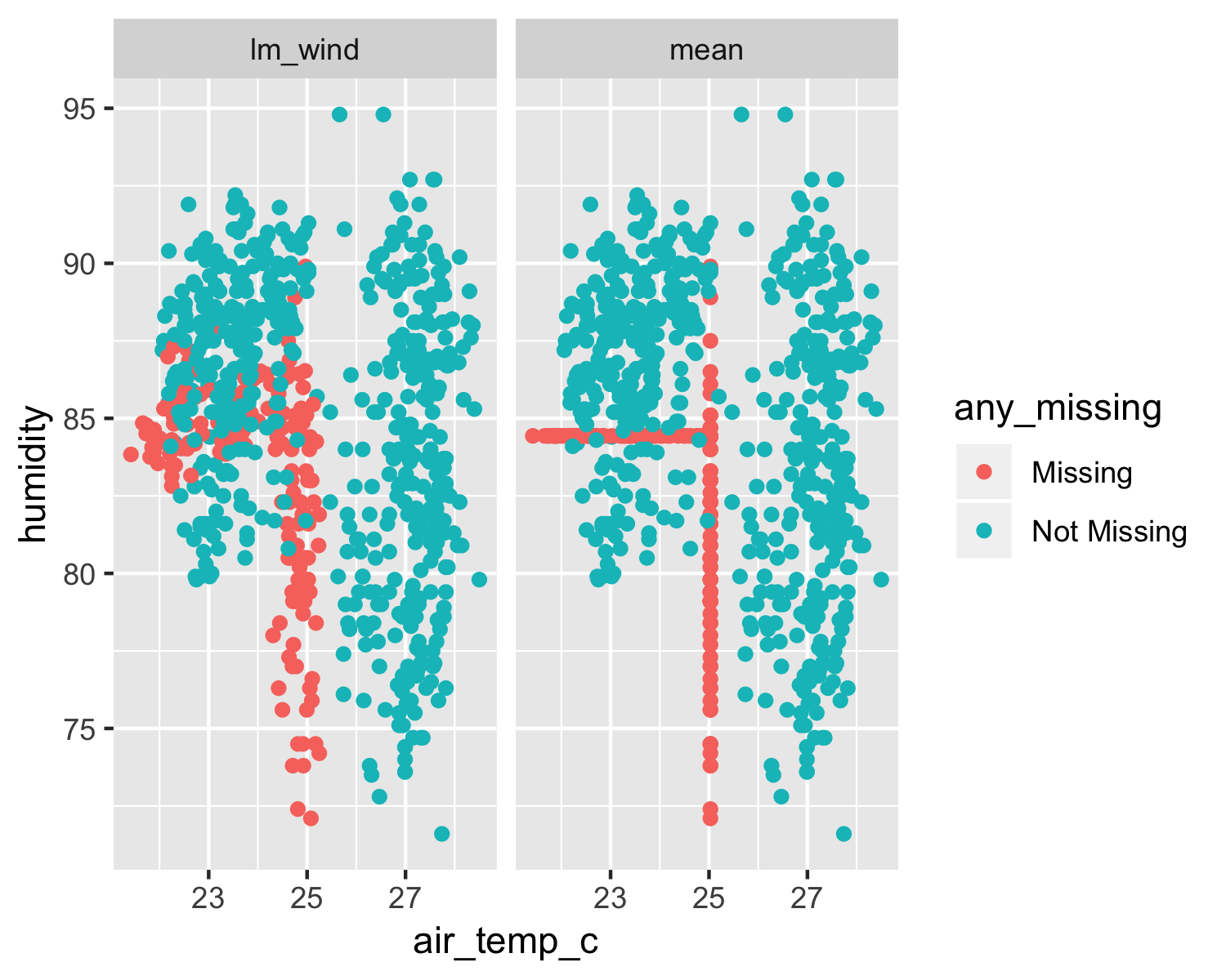
naniar::impute_mean_all()
simputation::impute_lm()

평균 대치 이미지

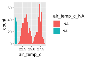
대치값과 원래 값 비교

ggplot(ocean_imp_track, 
       aes(x = air_temp_c, 
           fill = air_temp_c_NA)) + 
  geom_histogram()

대치 히스토그램

챕터 4

여러 대치 모델 사용

선형모델 대치 vs 평균 대치 비교

대치 모델이 추론에 미치는 영향

# A tibble: 12 x 6
   imp_model term  estimate
   <chr>     <chr>    <dbl>
 1 cc        (Int… -7.35e+2
 2 cc        air_…  8.64e-1
 3 cc        humi…  3.41e-2
 4 cc        year   3.69e-1
 5 imp_lm_w… (Int… -1.71e+3
 6 imp_lm_w… air_…  3.78e-1
# ... 6 more rows
# ... with 3 more variables:
#   std.error <dbl>,
#   statistic <dbl>,
#   p.value <dbl>

이제 시작입니다!

naniar.njtierney.com

visdat.njtierney.com

mice R 패키지

Flexible Imputation of Missing Data

감사합니다!

R에서 결측치 다루기