R로 배우는 Feature Engineering
Jorge Zazueta
Research Professor. Head of the Modeling Group at the School of Economics, UASLP
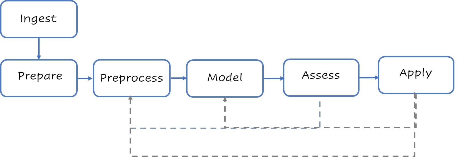
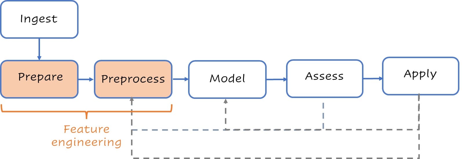
전형적인 고수준 모델링 단계입니다.

전형적인 고수준 모델링 단계입니다.

기본 정리와 데이터 분할을 먼저 수행합니다.
loans <- # Basic housekeeping
loans %>%
mutate(across(where(is_character),
as_factor)) %>%
mutate(across(Credit_History,
as_factor))
set.seed(123) # Set up splits
split <- initial_split(loans,
strata = Loan_Status)
test <- testing(split)
train <- training(split)
glimpse(train)
Rows: 460
Columns: 13
$ Loan_ID <fct> LP001003...
$ Gender <fct> Male, Ma...
$ Married <fct> Yes, No,...
$ Dependents <fct> 1, 0, 0,...
$ Education <fct> Graduate...
$ Self_Employed <fct> No, No, ...
$ ApplicantIncome <dbl> 4583, 18...
$ CoapplicantIncome <dbl> 1508, 28...
$ LoanAmount <dbl> 128, 114...
$ Loan_Amount_Term <dbl> 360, 360...
$ Credit_History <fct> 1, 1, 0,...
$ Property_Area <fct> Rural, R...
$ Loan_Status <fct> N, N, N,...
레시피는 간단할 수도, 매우 복잡할 수도 있습니다.
recipe <- recipe(Loan_Status ~ .,
data = train) %>%
update_role(Loan_ID,
new_role = "ID") %>%
step_normalize(all_numeric_predictors()) %>%
step_impute_knn(all_predictors()) %>%
step_dummy(all_nominal_predictors())
recipe
Recipe
Inputs:
role #variables
ID 1
outcome 1
predictor 11
Operations:
Centering and scaling for all_numeric_predictors()
K-nearest neighbor imputation for all_predictors()
Dummy variables from all_nominal_predictors()
워크플로 설정
lr_model <- logistic_reg() %>%
set_engine("glmnet") %>%
set_args(mixture = 1, penalty = tune())
lr_penalty_grid <- grid_regular(
penalty(range = c(-3, 1)),
levels = 30)
lr_workflow <-
workflow() %>%
add_model(lr_model) %>%
add_recipe(recipe)
lr_workflow
--Workflow -------------------------------
Preprocessor: Recipe
Model: logistic_reg()
-- Preprocessor --------------------------
3 Recipe Steps
- step_normalize()
- step_impute_knn()
- step_dummy()
-- Model ---------------------------------
로지스틱 회귀 모델 사양(분류)
주요 인자:
penalty = tune()
mixture = 1
계산 엔진: glmnet
Lasso 패널티 튜닝
lr_tune_output <- tune_grid(
lr_workflow,
resamples = vfold_cv(train, v = 5),
metrics = metric_set(roc_auc),
grid = penalty_grid)
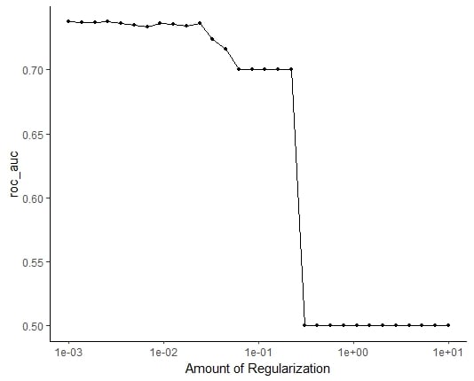
autoplot(tune_output)
ROC_AUC vs. 정규화

최종 모델 적합
best_penalty <-
select_by_one_std_err(lr_tune_output,
metric = 'roc_auc', desc(penalty))
lr_final_fit<-
finalize_workflow(lr_workflow, best_penalty) %>%
fit(data = train)
lr_final_fit %>%
augment(test) %>%
class_evaluate(truth = Loan_Status,
estimate = .pred_class,
.pred_Y)
성능 지표
# A tibble: 2 × 3
.metric .estimator .estimate
<chr> <chr> <dbl>
1 accuracy binary 0.818
2 roc_auc binary 0.813
R로 배우는 Feature Engineering