차원 축소

R로 배우는 Feature Engineering

Jorge Zazueta

Research Professor and Head of the Modeling Group at the School of Economics, UASLP

zero-variance 특성

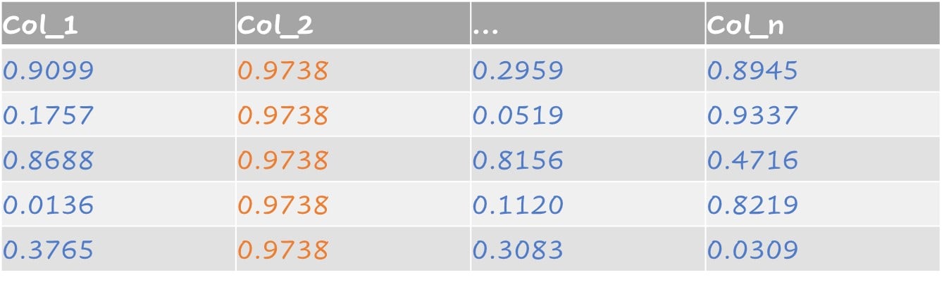
일부 데이터셋에는 상수값 또는 분산이 0인 열이 있습니다. recipe()에 step_zv()를 추가하여 이러한 특성을 제거할 수 있습니다.

분산이 0인 특성을 보여주는 표.

near-zero-variance 특성

near-zero-variance 특성에는 단일 값인 예측자뿐 아니라 아래 두 가지를 모두 만족하는 예측자가 포함됩니다:

표본 수에 비해 고유값 개수가 매우 적음
최빈값의 빈도와 두 번째로 흔한 값의 빈도 비율이 큼

near-zero-variance 예:

관측치 100개에서 서로 다른 값이 2개뿐이고, 그중 하나는 한 번만 나타남.

step_nzv()는 이러한 예측자를 식별해 제거합니다.

주성분분석(PCA)

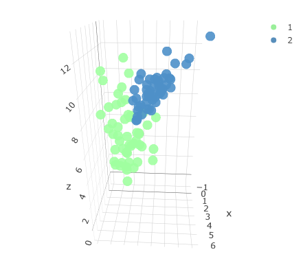
두 개의 클래스가 있는 원래 3차원 데이터셋.

두 데이터 클래스를 가진 3차원 그래프.

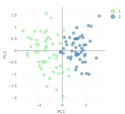
첫 두 주성분으로 표현한 축소 데이터셋.

첫 두 주성분의 산점도로 두 데이터 클래스를 보여주는 2차원 그래프.

레시피 준비하기

PCA를 수행하는 recipe를 만들고 prep()으로 결과를 가져옵니다.

pc_recipe <- 
recipe(~., data = loans_num) %>%
  step_nzv(all_numeric()) %>%
  step_normalize(all_numeric()) %>%
  step_pca(all_numeric())

pca_output <- prep(pc_recipe)

pca_output에 대해 names()를 호출해 이용 가능한 정보를 확인합니다.

names(pca_output)

 [1] "var_info"       "term_info"     
 [3] "steps"          "template"      
 [5] "levels"         "retained"      
 [7] "requirements"   "tr_info"       
 [9] "orig_lvls"      "last_term_info"

설명분산 살펴보기

pca_output 객체에서 표준편차를 추출하고 설명분산을 계산합니다.

stdv <- pca_output$steps[[3]]$res$sdev

var_explained <- stdv^2/sum(stdv^2)

PCA = tibble(PC = 1:length(stdv),
          var_explained = var_explained, 
          cumulative = cumsum(var_explained))

주성분별 설명분산을 보여주는 표입니다.

# A tibble: 5 × 3
     PC var_explained cumulative
  <int>         <dbl>      <dbl>
1     1        0.315       0.315
2     2        0.214       0.529
3     3        0.202       0.730
4     4        0.198       0.928
5     5        0.0722      1

설명분산 시각화

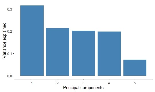
ggplot2로 막대 그래프로 시각화할 수 있습니다.

PCA %>% 
ggplot(aes(x = PC, 
           y = var_explained)) +
  geom_col(fill = "steelblue") +
  xlab("Principal components") +
  ylab("Variance explained")

주성분별 설명분산.

주성분별 설명분산을 보여주는 막대 그래프.

연습해 봅시다!

R로 배우는 Feature Engineering