Python으로 설계하는 Machine Learning 워크플로
Dr. Chris Anagnostopoulos
Honorary Associate Professor
clf = GaussianNB().fit(X_train, y_train)
scores = clf.predict_proba(X_test)
array([[3.74717371e-07, 9.99999625e-01],
       [9.99943716e-01, 5.62841678e-05],
       ...,
       [9.99937502e-01, 6.24977552e-05]])
[s[1] > 0.5 for s in scores] == clf.predict(X_test)
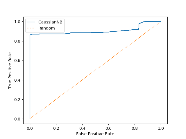
fpr, tpr, thres = roc_curve(
    ground_truth,
    [s[1] for s in scores])
plt.plot(fpr, tpr)
plt.xlabel('False Positive Rate')
plt.ylabel('True Positive Rate')
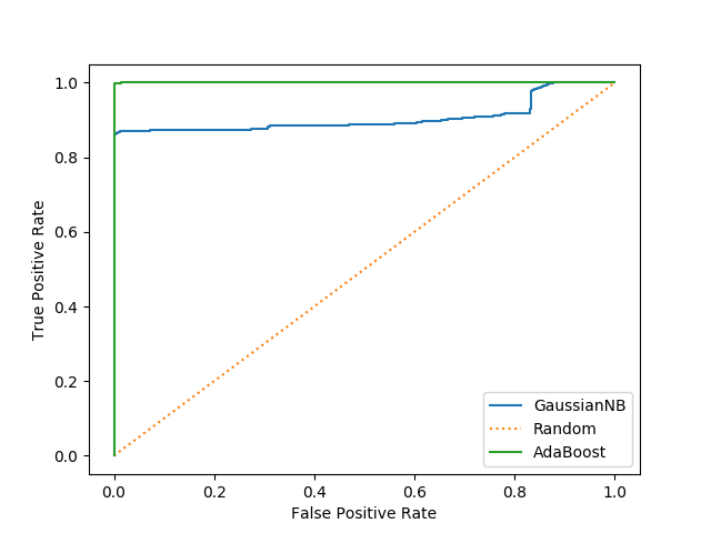
clf = AdaBoostClassifier().fit(X_train, y_train)
scores_ab = clf.predict_proba(X_test)
roc_auc_score(ground_truth, [s[1] for s in scores_ab])
0.9999
def my_scorer(y_test, y_est, cost_fp=10.0, cost_fn=1.0):
    tn, fp, fn, tp = confusion_matrix(y_test, y_est).ravel()
    return cost_fp*fp + cost_fn*fn
t_range = [0.0, 0.25, 0.5, 0.75, 1.0]
costs = [
   my_scorer(y_test, [s[1] > thres for s in scores]) for thres in t_range
]
[94740.0, 626.0, 587.0, 507.0, 2855.0]