R로 기술통계

SAS 사용자를 위한 R

Melinda Higgins, PhD

Research Professor/Senior Biostatistician Emory University

외부 CSV 데이터셋 불러오기

  • Abalone 데이터셋에는 9개 측정값이 있습니다:
    • length
    • diameter
    • height
    • whole weight
    • shucked weight
    • shell weight
    • viscera weight
    • sex (유생, 암컷, 수컷)
    • rings 수

전복 사진

  • 총 4177개 전복
SAS 사용자를 위한 R

외부 CSV 데이터셋 불러오기

  • abalone 데이터셋은 CSV(쉼표로 구분된 값) 형식입니다
  • readr 패키지의 read_csv()로 CSV를 불러옵니다

readr 헥스스티커 로고

SAS 사용자를 위한 R

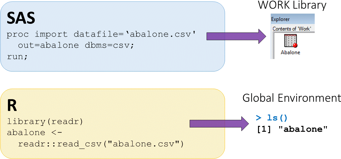
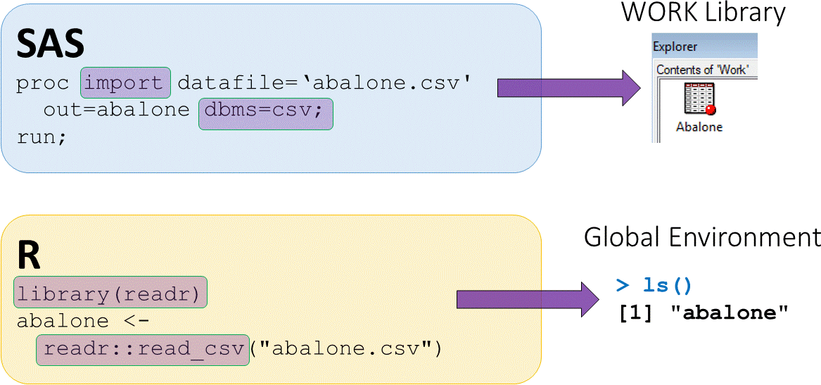
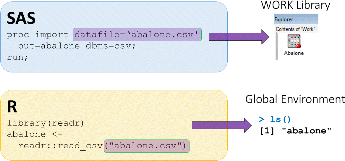
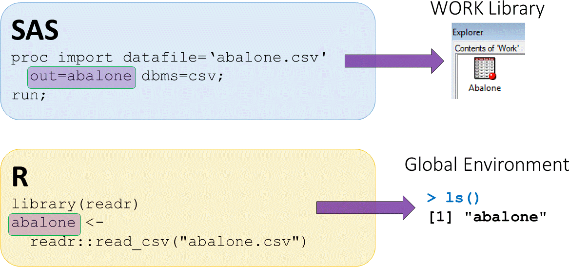
readr의 read_csv 사용 예: SAS PROC IMPORT과 유사

SAS 사용자를 위한 R

readr 패키지의 read_csv 함수와 유사한 SAS PROC IMPORT

SAS 사용자를 위한 R

readr 패키지의 read_csv 함수와 유사한 SAS PROC IMPORT

SAS 사용자를 위한 R

readr 패키지의 read_csv 함수와 유사한 SAS PROC IMPORT

  • 할당 연산자 <-readr::read_csv의 출력을 객체 abalone에 저장합니다
  • abalone은 이제 전역 환경에 저장됩니다
SAS 사용자를 위한 R

SAS PROC CONTENTS와 유사한 R str 구조 함수

str(abalone)
Classes ‘tbl_df’, ‘tbl’ and 'data.frame':    4177 obs. of  9 variables:
 $ sex          : chr  "M" "M" "F" "M" ...
 $ length       : num  0.455 0.35 0.53 0.44 0.33 0.425 0.53 0.545 ...
 $ diameter     : num  0.365 0.265 0.42 0.365 0.255 0.3 0.415 0.425  ...
 $ height       : num  0.095 0.09 0.135 0.125 0.08 0.095 0.15 0.125 ...
 $ wholeWeight  : num  0.514 0.226 0.677 0.516 0.205 ...
 $ shuckedWeight: num  0.2245 0.0995 0.2565 0.2155 0.0895 ...
 $ visceraWeight: num  0.101 0.0485 0.1415 0.114 0.0395 ...
 $ shellWeight  : num  0.15 0.07 0.21 0.155 0.055 0.12 0.33 0.26 ...
 $ rings        : int  15 7 9 10 7 8 20 16 9 19 ...

SAS 사용자를 위한 R

R의 dim과 names 함수로 PROC CONTENTS 유사 기능

# abalone 데이터셋의 차원 표시
dim(abalone)
4177    9
# abalone의 변수 이름    names(abalone)

"sex" "length" "diameter" "height" "wholeWeight" "shuckedWeight" "visceraWeight" "shellWeight" "rings"
SAS 사용자를 위한 R

데이터셋 내용과 변수 유형

  • head()tail()은 기본으로 위/아래 6행을 보여줍니다
  • 두 번째 인수로 표시할 행 수를 변경할 수 있습니다
# abalone의 아래쪽 7행 표시
tail(abalone, 7)
# A tibble: 7 x 9
  sex   length diameter height wholeWeight shuckedWeight visceraWeight shellWeight rings
  <chr>  <dbl>    <dbl>  <dbl>       <dbl>         <dbl>         <dbl>       <dbl> <dbl>
1 M      0.55     0.43   0.13        0.840         0.316         0.196       0.240    10
2 M      0.56     0.43   0.155       0.868         0.4           0.172       0.229     8
3 F      0.565    0.45   0.165       0.887         0.37          0.239       0.249    11
4 M      0.59     0.44   0.135       0.966         0.439         0.214       0.260    10
5 M      0.6      0.475  0.205       1.18          0.526         0.288       0.308     9
6 F      0.625    0.485  0.15        1.09          0.531         0.261       0.296    10
7 M      0.71     0.555  0.195       1.95          0.946         0.376       0.495    12
SAS 사용자를 위한 R

dplyr로 데이터 다루기

dplyr 헥스스티커 로고

이 강의에서는 다음 dplyr 함수를 사용합니다:

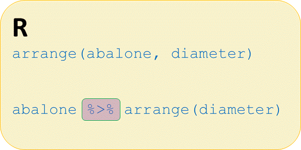
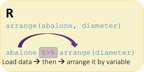
  • %>%dplyr에 포함된 magrittr의 파이프 연산자입니다
  • arrange()는 하나 이상의 변수로 정렬합니다
  • pull(x)는 열 x 하나를 추출합니다
  • select(x,y,z)는 여러 변수를 선택합니다
SAS 사용자를 위한 R

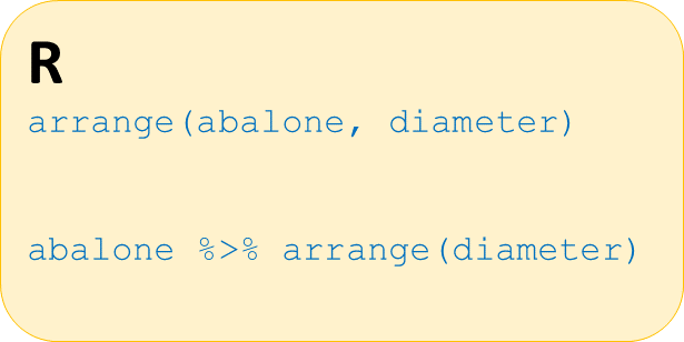
dplyr arrange와 파이프 %>%

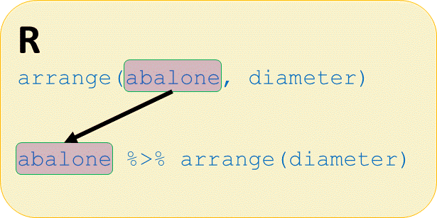
파이프 유무에 따른 r arrange 예시

SAS 사용자를 위한 R

dplyr arrange와 파이프 %>%

파이프 유무에 따른 r arrange 예시

SAS 사용자를 위한 R

dplyr arrange와 파이프 %>%

파이프 유무에 따른 r arrange 예시

SAS 사용자를 위한 R

dplyr arrange와 파이프 %>%

파이프 유무에 따른 r arrange 예시

SAS 사용자를 위한 R

지름으로 정렬하기

# abalone을 지름으로 정렬
abalone %>%
  arrange(diameter)
# A tibble: 4,177 x 9
   sex   length diameter height wholeWeight shuckedWeight visceraWeight shellWeight rings
   <chr>  <dbl>    <dbl>  <dbl>       <dbl>         <dbl>         <dbl>       <dbl> <dbl>
 1 I      0.075    0.055  0.01       0.002         0.001         0.0005      0.0015     1
 2 I      0.11     0.09   0.03       0.008         0.0025        0.002       0.003      3
 3 I      0.13     0.095  0.035      0.0105        0.005         0.0065      0.0035     4
 4 I      0.13     0.1    0.03       0.013         0.0045        0.003       0.004      3
 5 I      0.15     0.1    0.025      0.015         0.0045        0.004       0.005      2
 6 I      0.155    0.105  0.05       0.0175        0.005         0.0035      0.005      4
 7 I      0.14     0.105  0.035      0.014         0.0055        0.0025      0.004      3
 8 I      0.17     0.105  0.035      0.034         0.012         0.0085      0.005      4
 9 I      0.14     0.105  0.035      0.0145        0.005         0.0035      0.005      4
10 M      0.155    0.11   0.04       0.0155        0.0065        0.003       0.005      3
SAS 사용자를 위한 R

단일 변수 추출하기

dplyrpull()abalone에서 shuckedWeight를 추출해 보겠습니다

# abalone에서 shuckedWeight 변수만 추출
abalone %>%
  pull(shuckedWeight)
   [1] 0.2245 0.0995 0.2565 0.2155 0.0895 0.1410 0.2370 0.2940 0.2165 0.3145 0.1940 0.1675
  [13] 0.2175 0.2725 0.1675 0.2580 0.0950 0.1880 0.0970 0.1705 0.0955 0.0800 0.4275 0.3180
  [25] 0.5130 0.3825 0.3945 0.3560 0.3940 0.3930 0.3935 0.6055 0.5515 0.8150 0.6330 0.2270
  [37] 0.5305 0.2370 0.3810 0.1340 0.1865 0.3620 0.0315 0.0255 0.0175 0.0875 0.2930 0.1775
  [49] 0.0755 0.3545 0.2385 0.1335 0.2595 0.2105 0.1730 0.2565 0.1920 0.2765 0.0420 0.2460
  [61] 0.1800 0.3050 0.3020 0.1705 0.2340 0.2340 0.3540 0.4160 0.2135 0.0630 0.2640 0.1405
  [73] 0.4800 0.4740 0.4810 0.4425 0.3625 0.3630 0.2820 0.4695 0.3845 0.5105 0.3960 0.4080
  [85] 0.3800 0.3390 0.4825 0.3305 0.2205 0.3135 0.3410 0.3070 0.4015 0.5070 0.5880 0.5755
  [97] 0.2690 0.2140 0.2010 0.2775 0.1050 0.3280 0.3160 0.3105 0.4975 0.2910 0.2935 0.2610
...remaining output removed...
SAS 사용자를 위한 R

꺼낸 무게의 평균·중앙값 계산

# shuckedWeight의 평균 계산
abalone %>%
  pull(shuckedWeight) %>%
  mean()
0.3593675
# shuckedWeight의 중앙값 계산
abalone %>%
  pull(shuckedWeight) %>%
  median()
0.336
SAS 사용자를 위한 R

두 변수 선택하기

# length와 height 두 변수 선택
abalone %>%
  select(length, height)
# A tibble: 4,177 x 2
   length height
    <dbl>  <dbl>
 1  0.455  0.095
 2  0.35   0.09
 3  0.53   0.135
 4  0.44   0.125
 5  0.33   0.08
 6  0.425  0.095
 7  0.53   0.15
 8  0.545  0.125
# ... with 4,169 more rows
SAS 사용자를 위한 R

요약 통계 구하기: length, height

summary()는 최소, 최대, 평균, 중앙값, 1사분위수와 3사분위수를 출력합니다

# length와 height의 요약 통계
a balone %>%
  select(length, height) %>%
  summary()
     length          height      
 Min.   :0.075   Min.   :0.0000  
 1st Qu.:0.450   1st Qu.:0.1150  
 Median :0.545   Median :0.1400  
 Mean   :0.524   Mean   :0.1395  
 3rd Qu.:0.615   3rd Qu.:0.1650  
 Max.   :0.815   Max.   :1.1300
SAS 사용자를 위한 R

전복 데이터 살펴보기로 가봅시다

SAS 사용자를 위한 R

Preparing Video For Download...