선형 SVM 시각화

R에서의 Support Vector Machine

Kailash Awati

Instructor

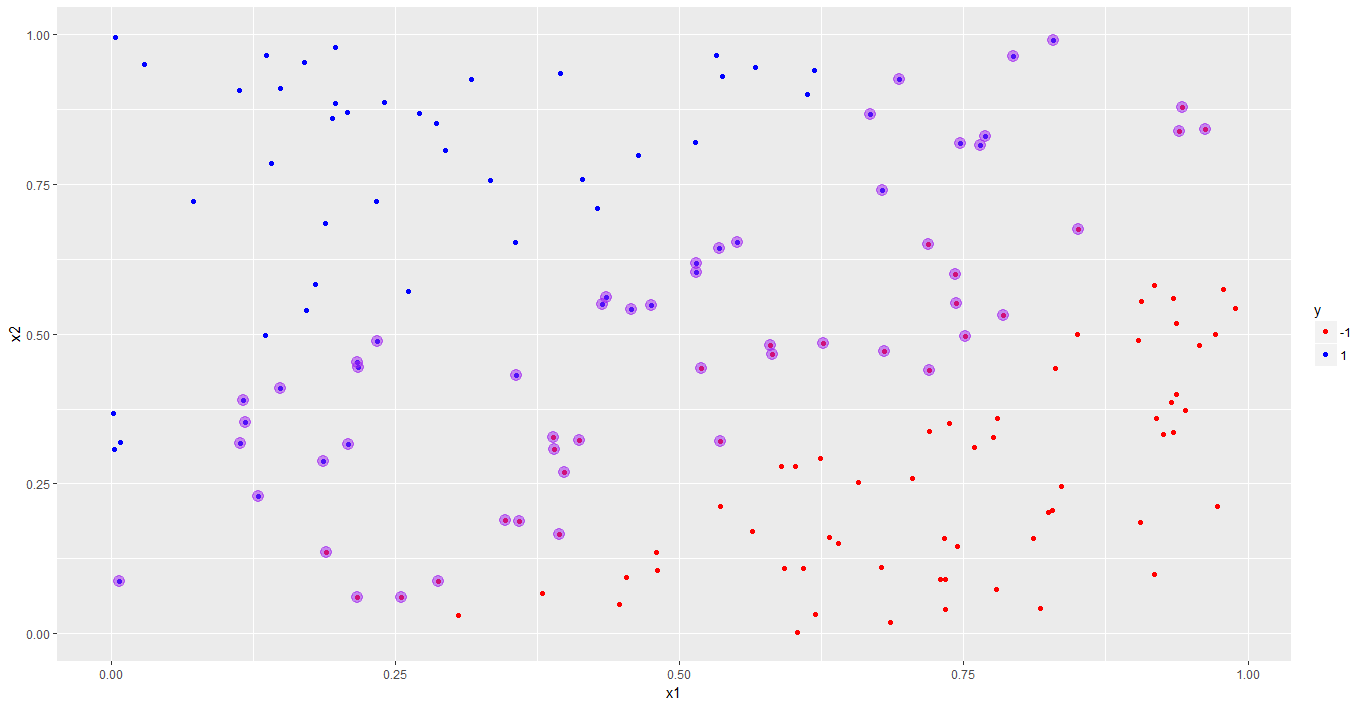
ggplot()으로 훈련 데이터를 시각화합니다.

# Visualize training data, distinguish classes using color
p <- ggplot(data = trainset, aes(x = x1, y = x2, color = y)) +
     geom_point() +
     scale_color_manual(values = c("red", "blue"))
# Render plot
p

svm_model의 index로 서포트 벡터를 표시합니다.

# Identify support vectors
df_sv <- trainset[svm_model$index, ]
# Mark out support vectors in plot
p <- p + geom_point(data = df_sv,
                    aes(x = x1, y = x2),
                    color = "purple",
                    size = 4, alpha = 0.5)
# Display plot
p

선형 분리 가능 데이터, 기본 비용 선형 커널 및 서포트 벡터

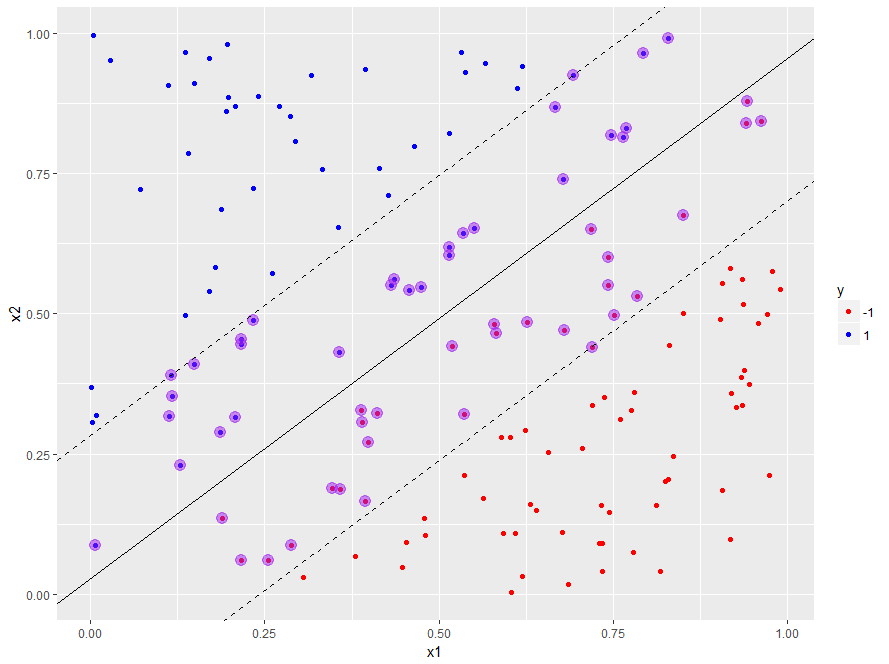
경계의 기울기와 절편 구하기:

svm_model의 coefs와 SV로 가중치 벡터 w 구성.

# Build weight vector
w <- t(svm_model$coefs) %*% svm_model$SV

기울기 =-w[1] / w[2]

# Calculate slope and save it to a variable
slope_1 <- -w[1] / w[2]

절편 = svm_model$rho / w[2]

# Calculate intercept and save it to a variable
intercept_1 <- svm_model$rho / w[2]

이전 슬라이드에서 계산한 기울기와 절편으로 결정 경계를 추가합니다.
geom_abline()을 사용하여 결정 경계를 플롯에 추가합니다.

# Plot decision boundary based on calculated slope and intercept
p <- p + geom_abline(slope = slope_1,
                     intercept = intercept_1)

마진은 결정 경계에 평행하며, 양쪽으로 1 / w[2]만큼 이동합니다.

# Add margins to plot
p <- p + 
    geom_abline(slope = slope_1,
                intercept = intercept_1 - 1 / w[2],
                linetype = "dashed") + 
    geom_abline(slope = slope_1,
                intercept = intercept_1 + 1 / w[2],
                linetype = "dashed")
# Display plot
p

선형 분리 가능 데이터, 기본 비용 선형 커널, 서포트 벡터 및 결정·마진 경계 시각화

소프트 마진 분류기

경계의 위치/형태에 불확실성 허용
- 완전히 선형인 경우는 없음
- 대개 알 수 없음
결정 경계가 선형이므로 마진 축소 가능

svm plot() 함수로 결정 경계 시각화

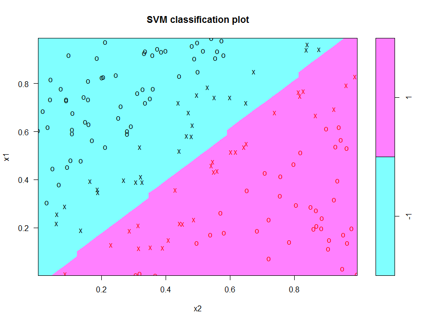
e1071의 plot() 함수를 사용하면 결정 경계를 쉽게 시각화할 수 있습니다.

# Visualize decision boundary using built in plot function
plot(x = svm_model,
     data = trainset)

선형 분리 가능 데이터셋, 기본 비용 선형 커널, svm.plot으로 시각화한 결정 경계

직접 연습해 보세요!

R에서의 Support Vector Machine