부트스트래핑을 활용한 다중 대치

R에서 대치(Imputation)로 결측치 다루기

Michal Oleszak

Machine Learning Engineer

대치로 인한 불확실성

대치는 일반적으로 분석/모델링 전 단계입니다.
결측값 추정에는 불확실성이 있습니다.
이 불확실성은 대치된 데이터로 수행하는 모든 분석에 반영되어야 합니다.

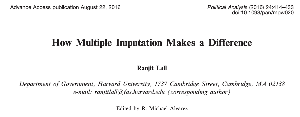
Ranjit Lall의 논문 "How Multiple Imputation Makes a Difference" 제목 페이지 머리말.

연구의 거의 절반에서 핵심 결과가 사라진다

부트스트랩

부트스트래핑 = 원래 크기의 데이터를 얻기 위해 행을 복원추출로 샘플링

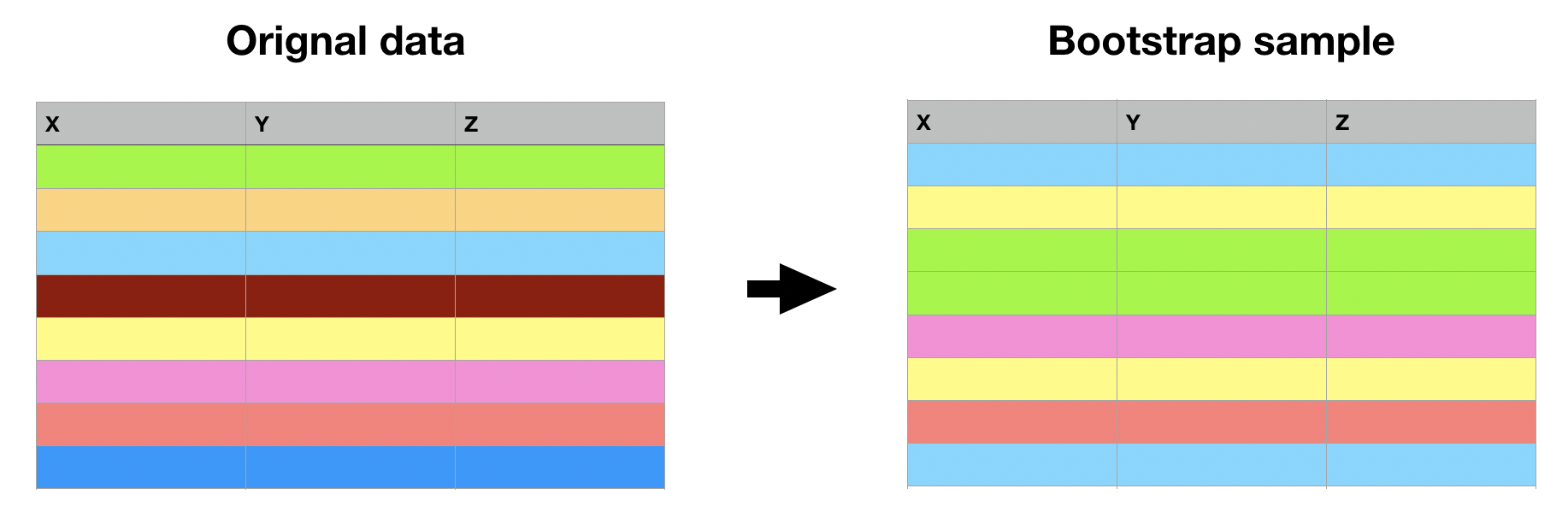
두 개의 모형 데이터 프레임. 왼쪽 "original data"에는 각 행이 다른 색으로 서로 다른 값을 표시합니다. 오른쪽 "bootstrapped sample"에는 "original data"의 일부 색 행이 여러 번 나타나고 일부는 전혀 없습니다.

부트스트래핑을 통한 다중 대치

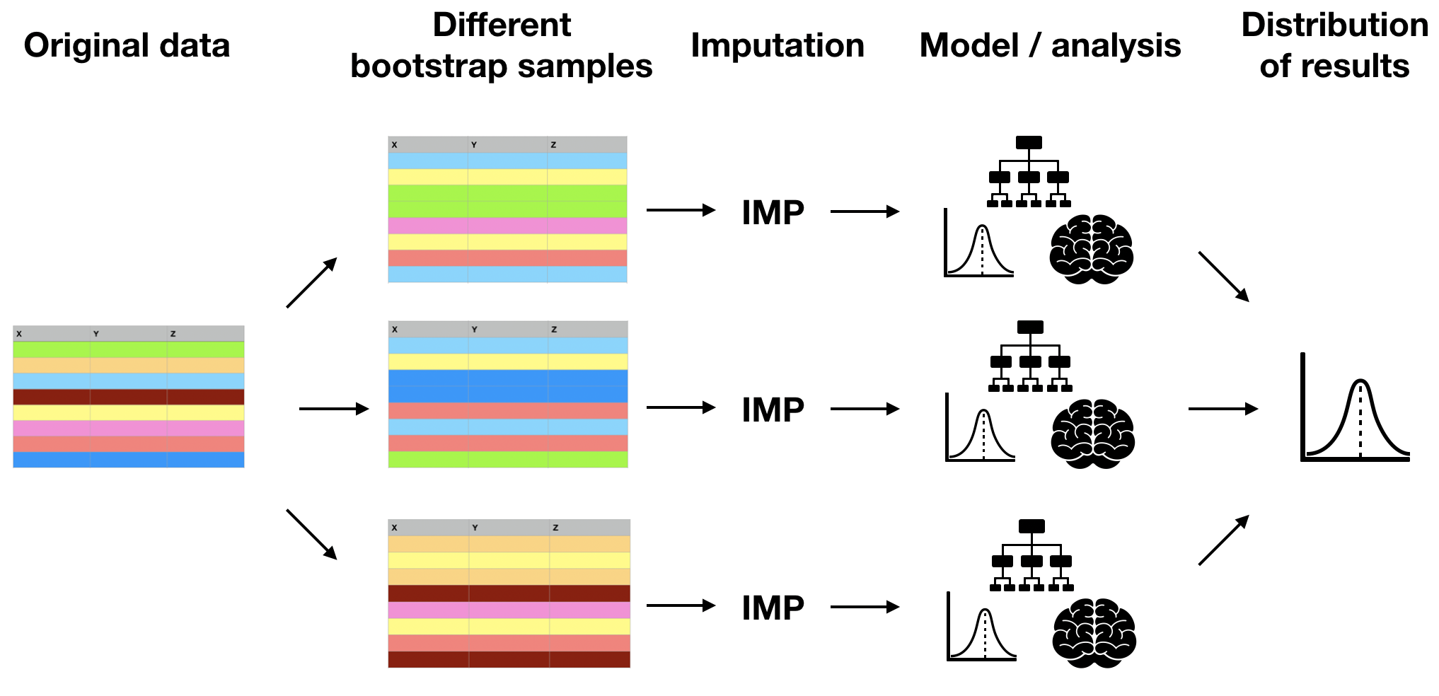
부트스트래핑으로 대치하는 5단계 다이어그램. "original data"에서 세 개의 화살표가 "different bootstrap samples"로 향합니다. 각 샘플에서 "Imputation"으로, 그다음 "Modeling / analysis"로, 마지막에 "Distribution of results"로 합쳐집니다.

부트스트랩 대치: 장단점

장점:

어떤 대치 방법과도 호환됩니다.
해석적으로 계산하기 어려운 양도 근사합니다.
MCAR, MAR 데이터 모두에 적용됩니다.

단점:

반복이 많거나 계산이 오래 걸리면 느립니다.

부트스트래핑 실습

calc_correlation <- function(data, indices) {






  # Return the correlation coefficient
  return(corr_coeff)
}

부트스트래핑 실습

calc_correlation <- function(data, indices) {
  # Get bootstrap sample
  data_boot <- data[indices, ]




  # Return the correlation coefficient
  return(corr_coeff)
}

부트스트래핑 실습

calc_correlation <- function(data, indices) {
  # Get bootstrap sample
  data_boot <- data[indices, ]
  # Impute with kNN imputation
  data_imp <- kNN(data_boot)


  # Return the correlation coefficient
  return(corr_coeff)
}

부트스트래핑 실습

calc_correlation <- function(data, indices) {
  # Get bootstrap sample
  data_boot <- data[indices, ]
  # Impute with kNN imputation
  data_imp <- kNN(data_boot)
  # Calculate correlation between Weight and TotChol
  corr_coeff <- cor(data_imp$Weight, data_imp$TotChol)
  # Return the correlation coefficient
  return(corr_coeff)
}

부트스트래핑 실습

library(boot)
boot_results <- boot(nhanes, statistic = calc_correlation, R = 50)
print(boot_results)

ORDINARY NONPARAMETRIC BOOTSTRAP

Call:
boot(data = nhanes, statistic = calc_correlation, R = 50)

Bootstrap Statistics :
      original      bias    std. error
t1* 0.03028306 0.007385452  0.04207152

부트스트랩 결과 시각화

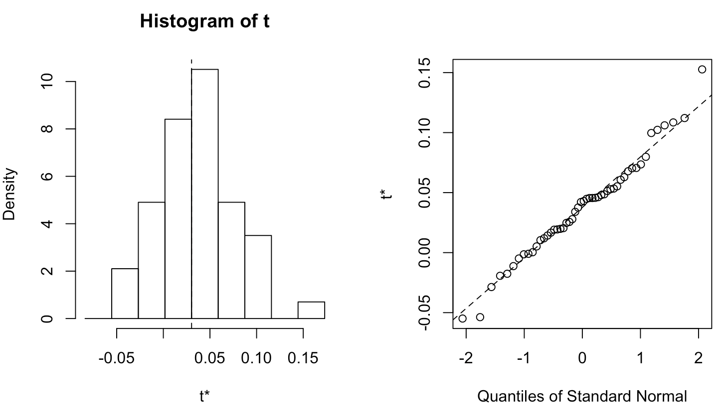
plot(boot_results)

부트스트랩 결과의 분포를 보여주는 히스토그램과 Q-Q 플롯. 둘 다 분포가 정규에 가깝다고 시사한다.

부트스트랩 신뢰구간

boot_ci <- boot.ci(boot_results, conf = 0.95, type = "norm")
print(boot_ci)

BOOTSTRAP CONFIDENCE INTERVAL CALCULATIONS
Based on 50 bootstrap replicates

CALL : 
boot.ci(boot.out = boot_results, conf = 0.95, type = "norm")

Intervals : 
Level      Normal        
95%   (-0.0596,  0.1054 )  
Calculations and Intervals on Original Scale

부트스트래핑을 연습해 봅시다!

R에서 대치(Imputation)로 결측치 다루기