데이터 모델링

R에서 limma로 하는 차등 발현 분석

John Blischak

Instructor

분석 준비 완료

# Plot principal components labeled by genotype
plotMDS(eset, labels = pData(eset)[, "genotype"], gene.selection = "common")
# Plot principal components labeled by treatment
plotMDS(eset, labels = pData(eset)[, "treatment"], gene.selection = "common")
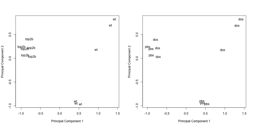
R에서 limma로 하는 차등 발현 분석

차등 발현 분석 단계

  • model.matrix로 디자인 행렬 구성

  • makeContrasts로 대비 행렬 구성

  • lmFit, contrasts.fit, eBayes로 대비 검정

R에서 limma로 하는 차등 발현 분석

독소루비신 연구의 그룹 평균 모델

$$ Y = \beta_1 X_1 + \beta_2 X_2 + \beta_3 X_3 + \beta_4 X_4 + \epsilon $$

  • $\beta_1$ - top2b 마우스의 dox 처리 평균 발현 수준
  • $\beta_2$ - top2b 마우스의 pbs 처리 평균 발현 수준
  • $\beta_3$ - wt 마우스의 dox 처리 평균 발현 수준
  • $\beta_4$ - wt 마우스의 pbs 처리 평균 발현 수준
R에서 limma로 하는 차등 발현 분석

독소루비신 연구의 대비

$\beta_1$ $\beta_2$ $\beta_3$ $\beta_4$
genotype top2b top2b wt wt
treatment dox pbs dox pbs
  • Response of wild type mice to dox treatment: $\beta_3 - \beta_4 = 0$

  • Response of Top2b null mice to dox treatment: $\beta_1 - \beta_2 = 0$

  • Differences between Top2b null and wild type mice in response to dox treatment: $(\beta_1 - \beta_2) - (\beta_3 - \beta_4) = 0$

R에서 limma로 하는 차등 발현 분석

독소루비신 연구 검정

  • lmFit으로 모델 계수 적합

  • contrasts.fit으로 대비 적합

  • eBayes로 t-통계량 계산

# Summarize results
results <- decideTests(fit2)
summary(results)
# Create a Venn diagram
vennDiagram(results)
R에서 limma로 하는 차등 발현 분석

연습해 봅시다!

R에서 limma로 하는 차등 발현 분석

Preparing Video For Download...