ACS의 오차 한계 시각화

R로 분석하는 미국 인구조사 데이터

Kyle Walker

Instructor

불확실성 시각화

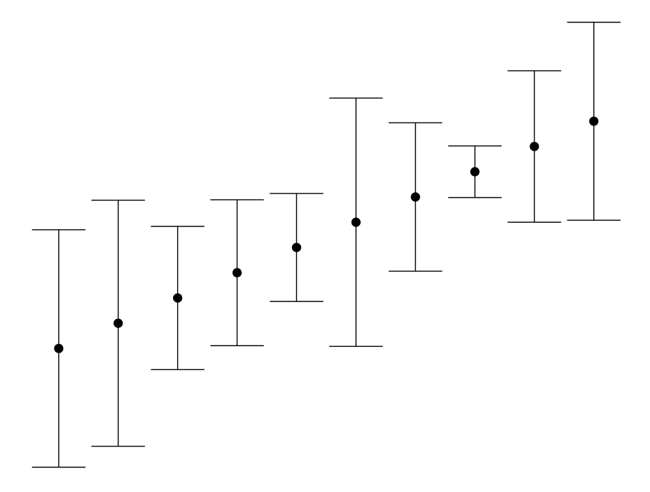
일반적인 방법: 오차 막대 그래프

오차 막대 그래프 예시

ggplot2에서 오차 한계 그래프

ggplot2에서: geom_errorbar() 및 geom_errorbarh()

library(tidycensus)
library(tidyverse)

wyoming_age <- get_acs(geography = "county", 
                       variables = c(medianage = "B01002_001"), 
                       state = "WY")  

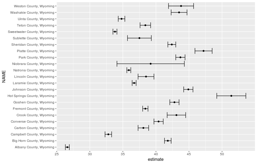
ggplot(wyoming_age, aes(x = estimate, y = NAME)) + 
  geom_errorbarh(aes(xmin = estimate - moe, 
                     xmax = estimate + moe)) + 
  geom_point()

서식 미적용 오차 한계 그래프

오차 한계 그래프 서식 지정

wyoming_age2 <- wyoming_age %>%
  mutate(NAME = str_replace(NAME, " County, Wyoming", ""))

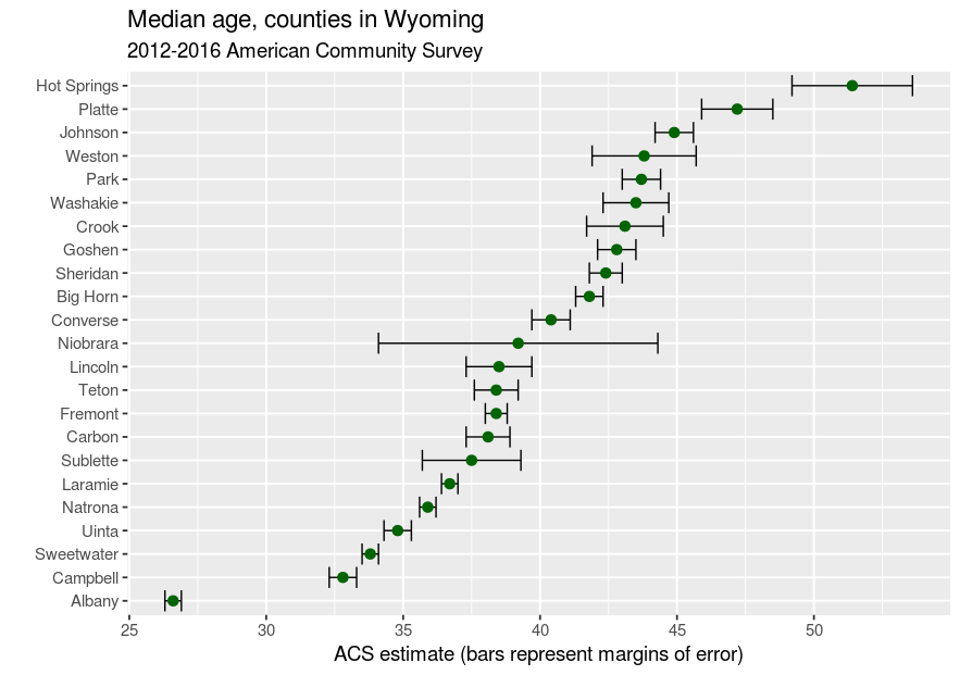
ggplot(wyoming_age2, 
       aes(x = estimate, 
           y = reorder(NAME, estimate))) + 
  geom_errorbarh(aes(xmin = estimate - moe, 
                     xmax = estimate + moe)) + 
  geom_point(size = 3, color = "darkgreen") + 
  theme_grey(base_size = 14) + 
  labs(title = "Median age, counties in Wyoming", 
       subtitle = "2012-2016 American Community Survey",
       x = "ACS estimate (bars represent margins of error)", 
       y = "")

서식 적용 오차 한계 그래프

연습해 봅시다!

R로 분석하는 미국 인구조사 데이터