R로 배우는 범주형 데이터 추론
Andrew Bray
Assistant Professor of Statistics at Reed College
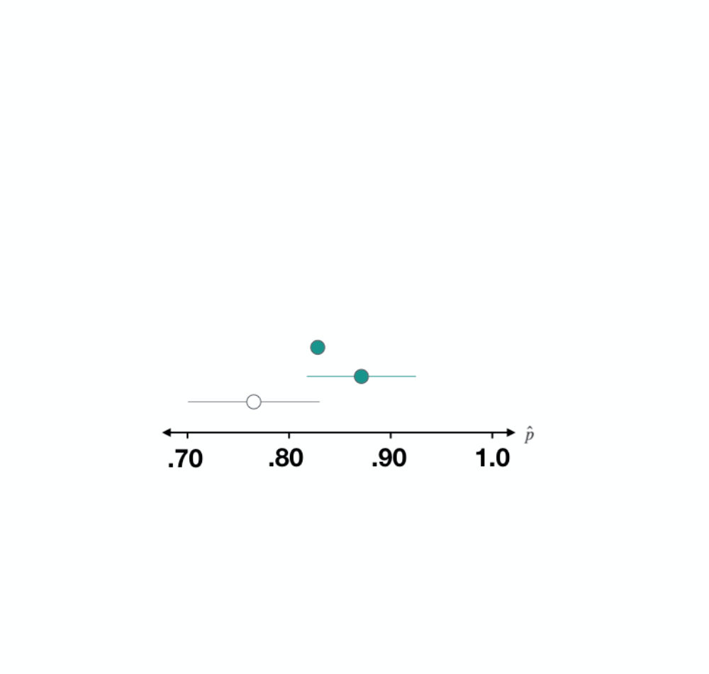
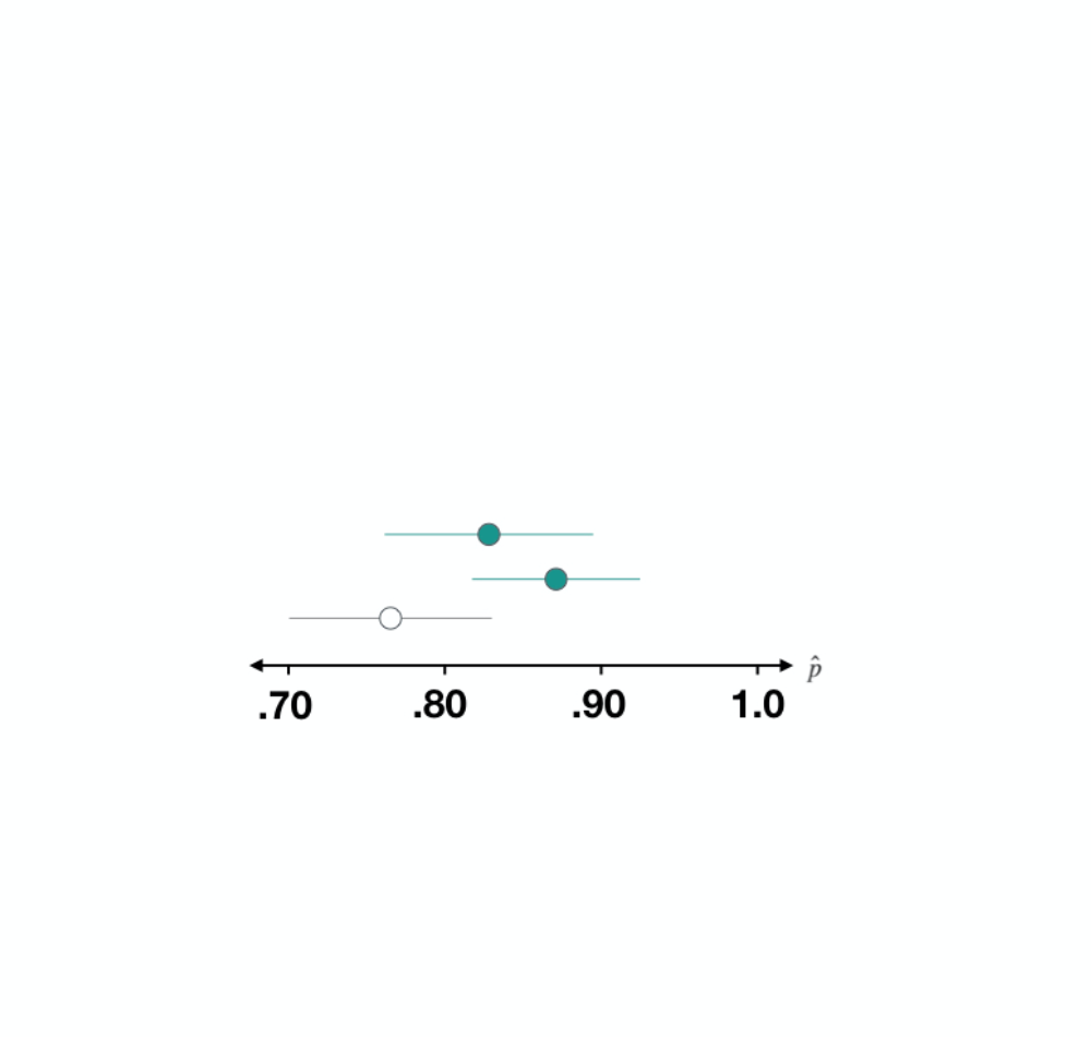
결론: 실제로 행복한 미국인의 비율은 0.705~0.841 사이입니다.
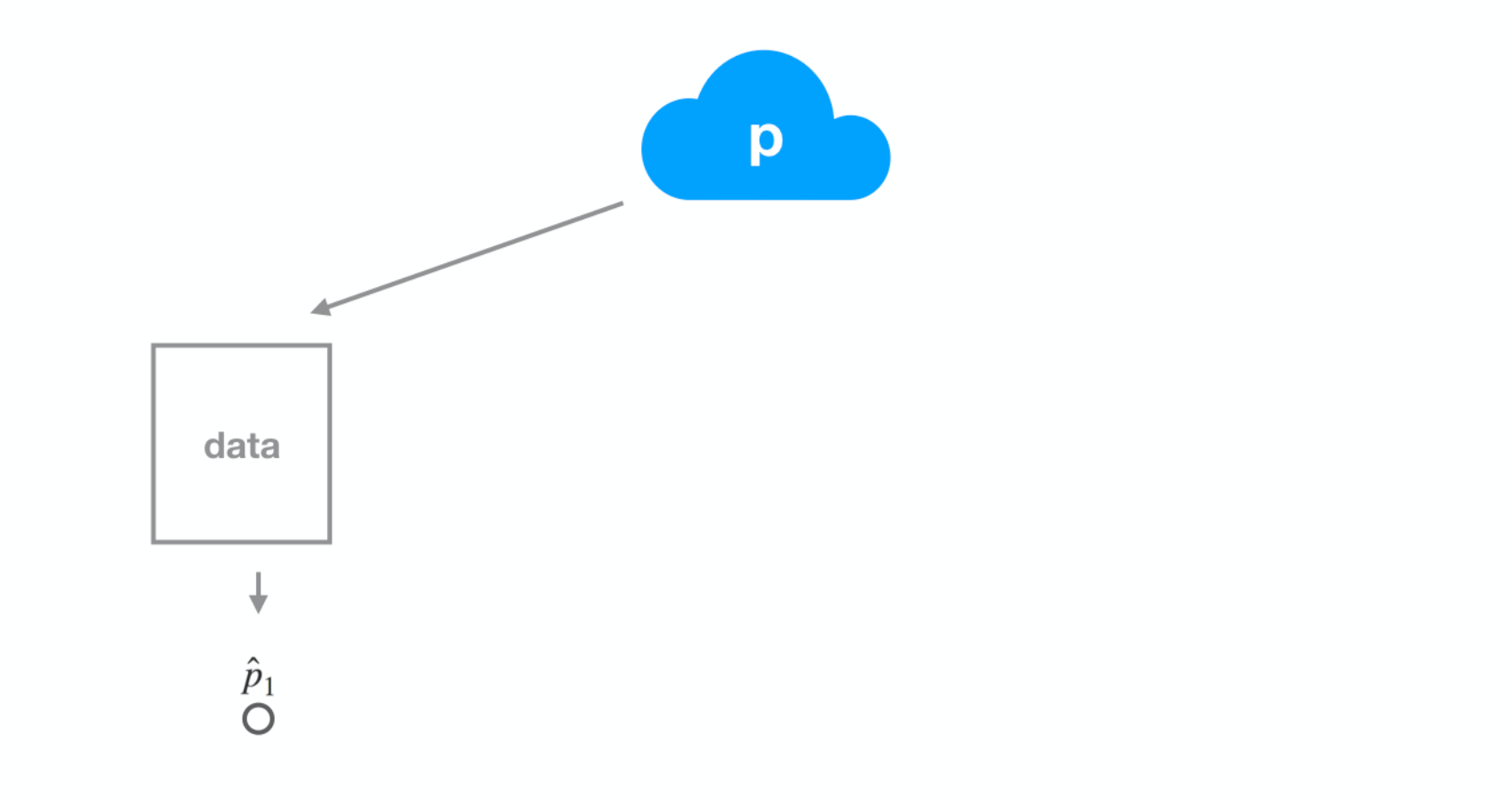
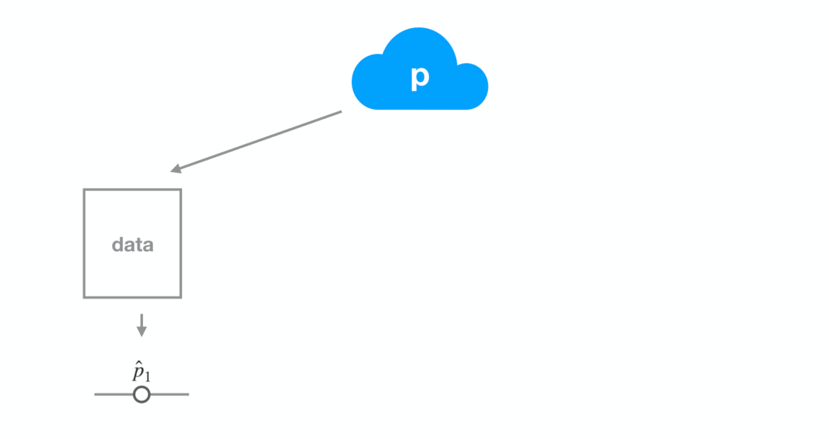
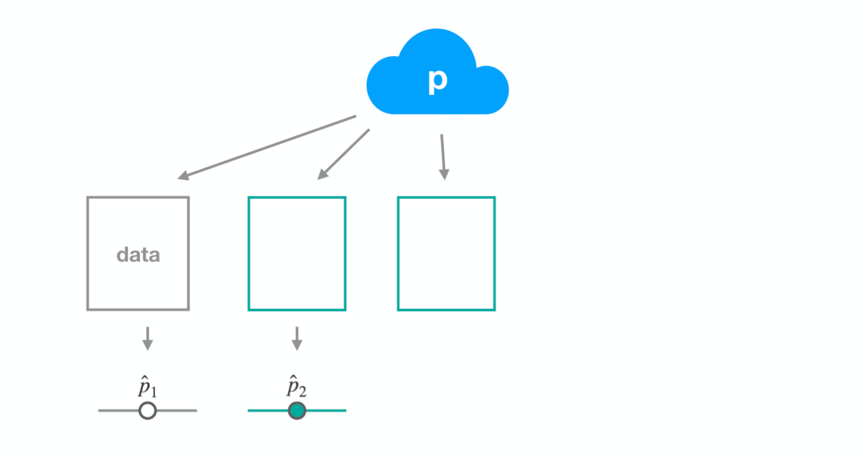
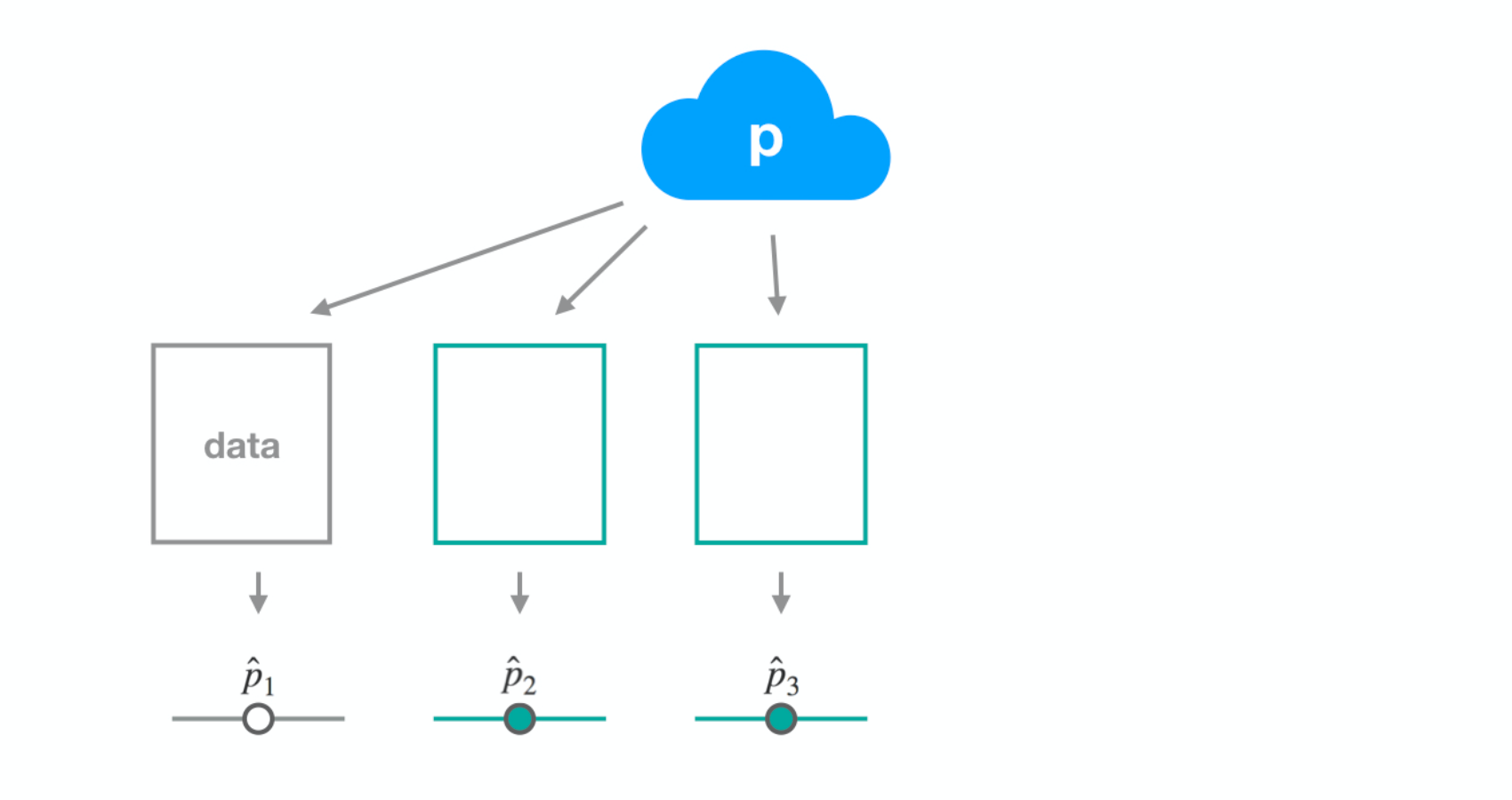
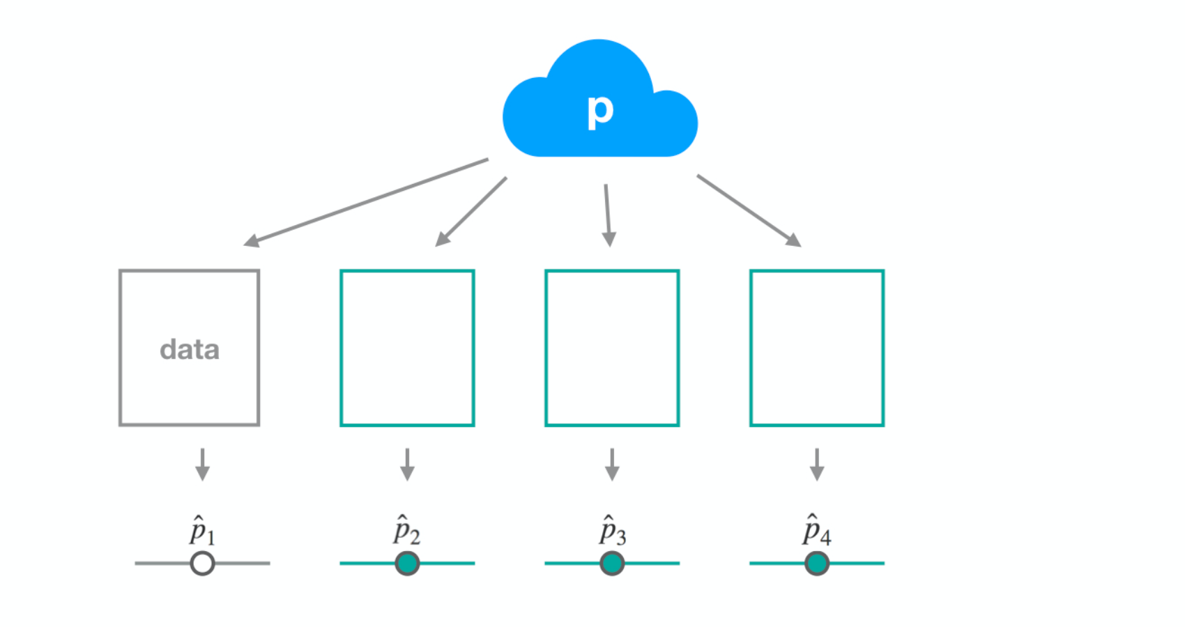
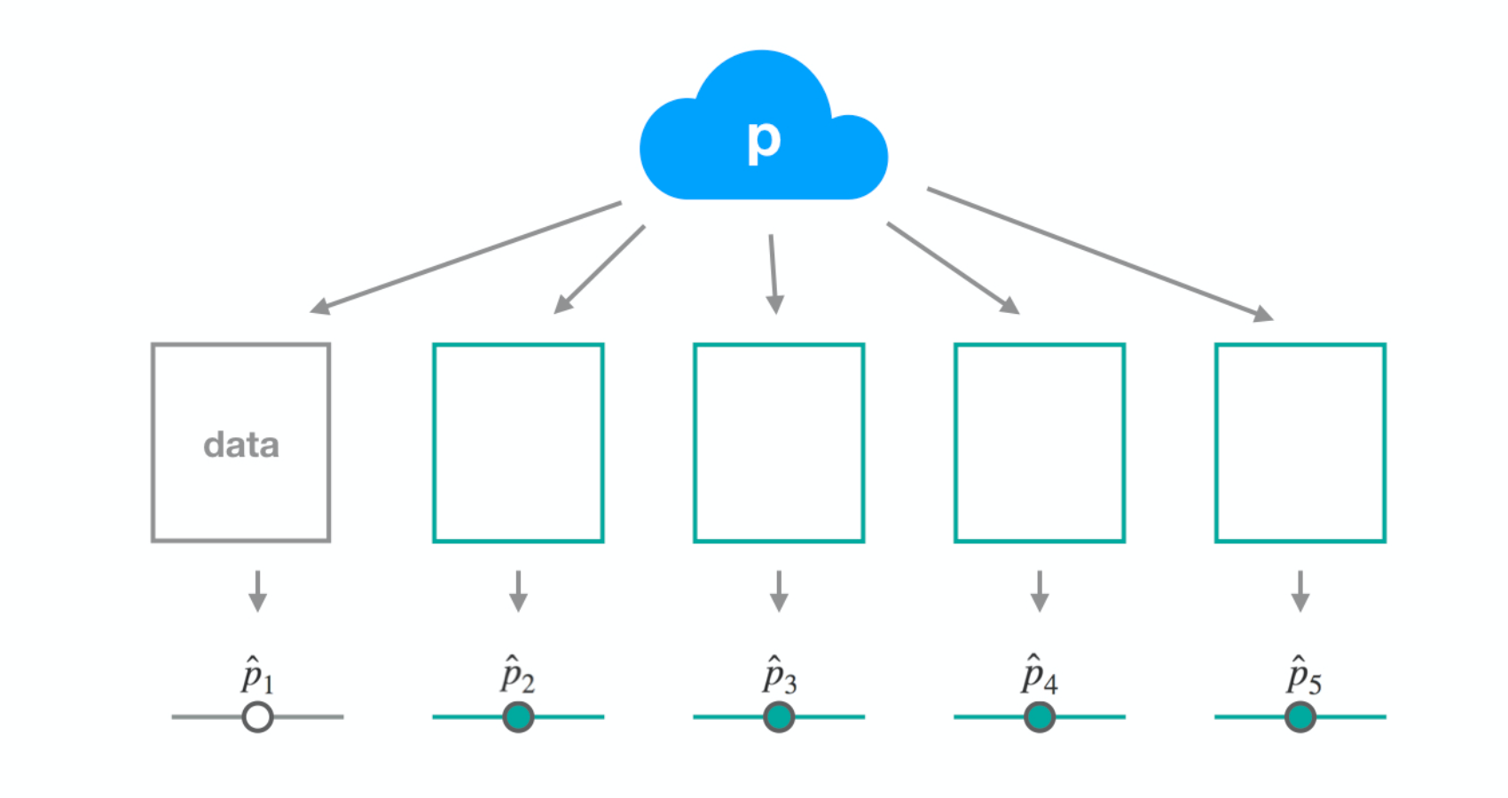
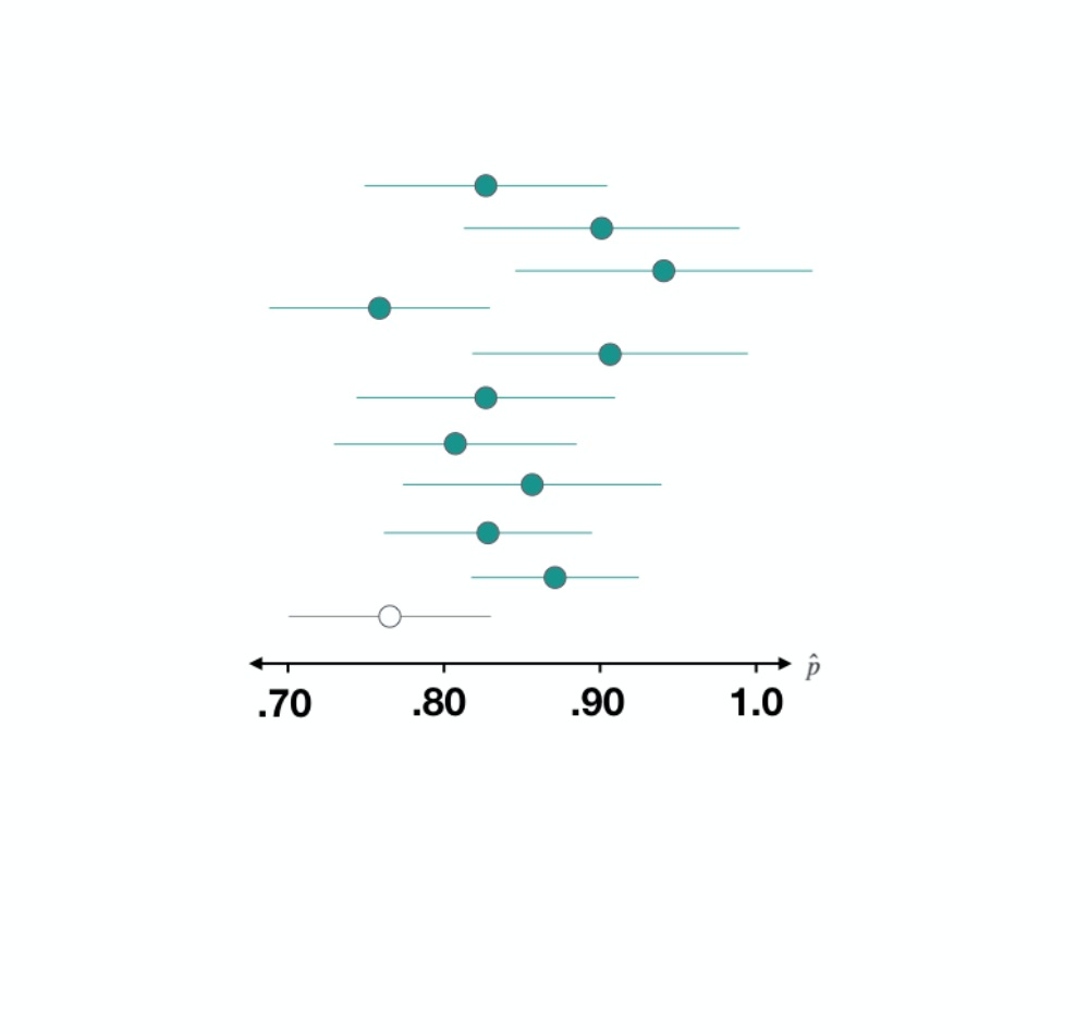
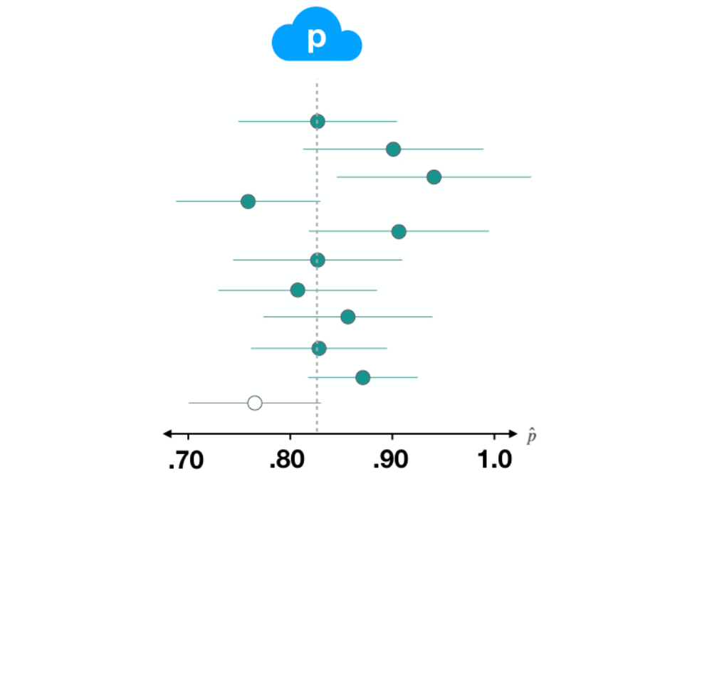
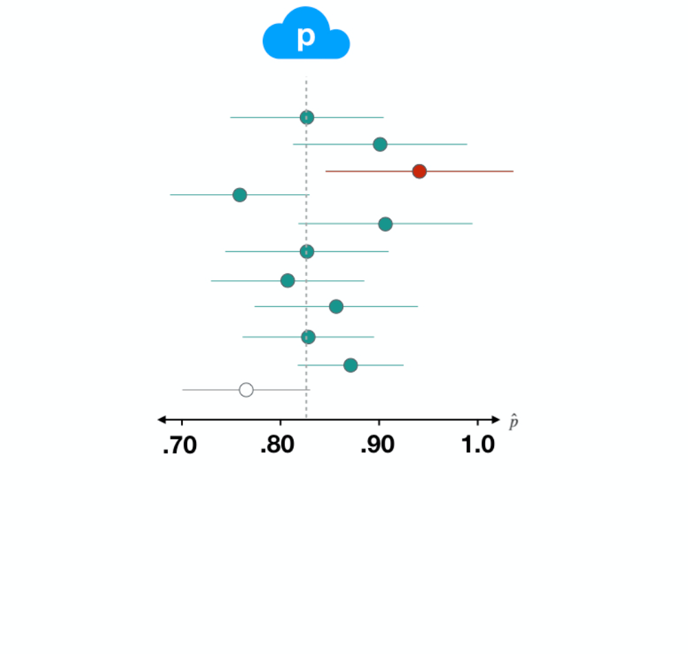
여기서 ‘신뢰’는 무엇을 뜻할까요?
ds1 <- filter(gss, year == 2016)

p_hat <- ds1 %>%
  summarize(mean(happy == "HAPPY")) %>%
  pull()

SE <- ds1 %>%
  specify(response = happy,
          success = "HAPPY") %>%
  generate(reps = 500,
           type = "bootstrap") %>%
  calculate(stat = "prop") %>%
  summarize(sd(stat)) %>%
  pull()

c(p_hat - 2 * SE, p_hat + 2 * SE)
ds1 <- filter(gss, year == 2016)
p_hat <- ds1 %>% summarize(mean(happy == "HAPPY")) %>% pull()
SE <- ds1 %>% specify(response = happy, success = "HAPPY") %>% generate(reps = 500, type = "bootstrap") %>% calculate(stat = "prop") %>% summarize(sd(stat)) %>% pull()
c(p_hat - 2 * SE, p_hat + 2 * SE)
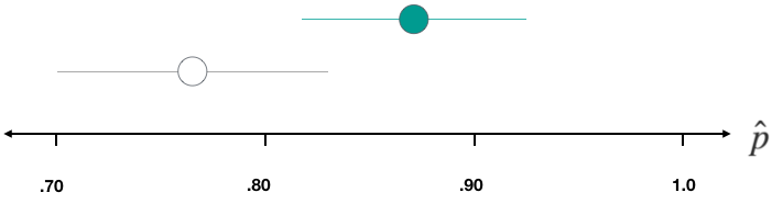
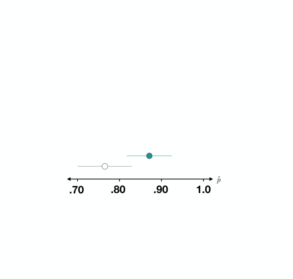
0.7073114 0.8393553
ds2 <- filter(gss, year == 2014)

p_hat <- ds1 %>%
  summarize(mean(happy == "HAPPY")) %>%
  pull()

SE <- ds1 %>%
  specify(response = happy,
          success = "HAPPY") %>%
  generate(reps = 500,
           type = "bootstrap") %>%
  calculate(stat = "prop") %>%
  summarize(sd(stat)) %>%
  pull()

c(p_hat - 2 * SE, p_hat + 2 * SE)
ds2 <- filter(gss, year == 2014)
0.8348831 0.9384503
ds3 <- filter(gss, year == 2012)

p_hat <- ds1 %>%
  summarize(mean(happy == "HAPPY")) %>%
  pull()

SE <- ds1 %>%
  specify(response = happy,
          success = "HAPPY") %>%
  generate(reps = 500,
           type = "bootstrap") %>%
  calculate(stat = "prop") %>%
  summarize(sd(stat)) %>%
  pull()

c(p_hat - 2 * SE, p_hat + 2 * SE)
ds3 <- filter(gss, year == 2012)
0.7626359 0.8906974
ds3 <- filter(gss, year == 2012)
p_hat <- ds3 %>%
  summarize(mean(happy == "HAPPY")) %>%
  pull()
SE <- ds3 %>%
  specify(response = happy,
          success = "HAPPY") %>%
  generate(reps = 500,
           type = "bootstrap") %>%
  calculate(stat = "prop") %>%
  summarize(sd(stat)) %>%
  pull()

c(p_hat - 2 * SE, p_hat + 2 * SE)
ds3 <- filter(gss, year == 2012) p_hat <- ds3 %>% summarize(mean(happy == "HAPPY")) %>% pull() SE <- ds3 %>% specify(response = happy, success = "HAPPY") %>% generate(reps = 500, type = "bootstrap") %>% calculate(stat = "prop") %>% summarize(sd(stat)) %>% pull()
해석: “행복한 미국인의 실제 비율이 0.705~0.841 사이라고 95% 신뢰합니다.”
구간의 너비에 영향을 주는 요인
n
p