대안 방법: 카이제곱 분포

R로 배우는 범주형 데이터 추론

Andrew Bray

Assistant Professor of Statistics at Reed College

근사 분포: 정규분포

통계량: $\hat{p}, \hat{p}_{1} - \hat{p}_{2}$

정규 분포 곡선

근사 분포: 카이제곱분포

통계량: $\hat{x}^{2}$
모양은 자유도에 의해 결정
$df = (nrows - 1) \times (ncols - 1)$

카이제곱 분포 곡선

근사에 의한 H-검정

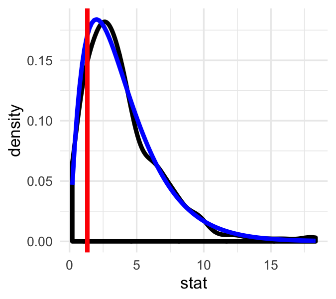
null_spac <- gss_party %>%
  specify(natspac ~ party) %>%
  hypothesize(null = "independence") %>%
  generate(reps = 100, type = "permute") %>%
  calculate(stat = "Chisq")

ggplot(null_spac, aes(x = stat)) +
  geom_density() +
  stat_function(
    fun = dchisq, 
    args = list(df = 4), 
    color = "blue"
  ) +
  geom_vline(xintercept = chi_obs_spac, color = "red")

근사에 의한 가설검정

근사에 의한 H-검정

gss_party %>%
  select(natarms, party) %>%
  table()

             party
natarms        D  I  R
  TOO LITTLE  17 20 24
  ABOUT RIGHT 14 28  8
  TOO MUCH    12 24  2

pchisq(chi_obs_spac, df = 4)

X-squared 
0.1430612

1 - pchisq(chi_obs_spac, df = 4)

X-squared 
0.8569388

근사에 의한 가설검정

카이제곱 분포

다음일 때 좋은 근사입니다:

$expected\_count >= 5$
$df >= 2$

카이제곱 분포 곡선

연습해 봅시다!

R로 배우는 범주형 데이터 추론