데이터셋에서 탐지 모델까지

R로 배우는 사기 탐지

Sebastiaan Höppner

PhD researcher in Data Science at KU Leuven

로드맵

(1) 데이터셋을 훈련 세트와 테스트 세트로 분할
(2) 머신 러닝 모델을 선택
(3) 클래스 분포 균형화를 위해 훈련 세트에 SMOTE 적용
(4) 재균형된 훈련 세트로 모델 학습
(5) (원본) 테스트 세트에서 성능 평가

훈련/테스트 세트로 분할

데이터셋을 훈련 세트와 테스트 세트로 분할(예: 50/50, 75/25 등)
처음에는 두 세트의 클래스 분포를 동일하게 유지
예: 50% 훈련, 50% 테스트

prop.table(table(train$Class))

   0    1 
0.98 0.02

prop.table(table(test$Class))

   0    1 
0.98 0.02

머신 러닝 모델 선택 및 학습

결정 트리, 인공 신경망, 서포트 벡터 머신, 로지스틱 회귀, 랜덤 포레스트, 나이브 베이즈, k-NN 등
예: CART(Classification And Regression Tree) 알고리즘
rpart 패키지의 rpart 함수

library(rpart)

model1 = rpart(Class ~ ., data = train)

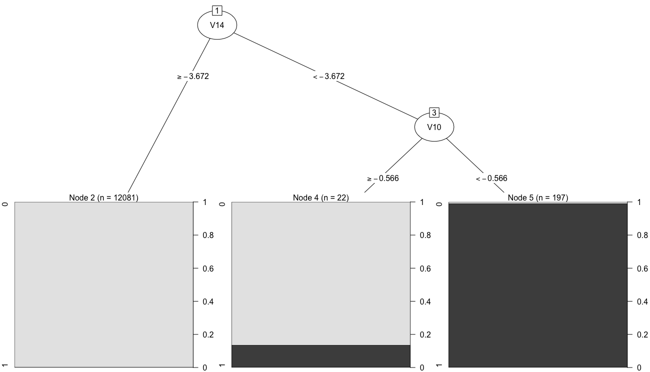
library(partykit)
plot(as.party(model1))

tree1

## 테스트 세트의 사기 확률 예측
scores1 = predict(model1, newdata = test, type = "prob")[, 2]

## 테스트 세트의 클래스(사기/정상) 예측
predicted_class1 = factor(ifelse(scores1 > 0.5, 1, 0))

## 혼동 행렬 & 정확도
library(caret)
CM1 = confusionMatrix(data = predicted_class1, reference = test$Class)

          Reference         
Prediction     0     1
         0 12046    55
         1     8   191       Accuracy : 0.994878

library(pROC)
auc(roc(response = test$Class, predictor = scores1)) ## ROC 곡선 하의 면적(AUC)

Area under the ROC curve: 0.8938

훈련 세트에 SMOTE 적용

library(smotefamily)
set.seed(123)

smote_result = SMOTE(X = train[, -17],
                     target = train$Class,
                     K = 5,
                     dup_size = 10)

train_oversampled = smote_result$data
colnames(train_oversampled)[17] = "Class"


prop.table(table(train_oversampled$Class))

        0         1 
0.8166667 0.1833333

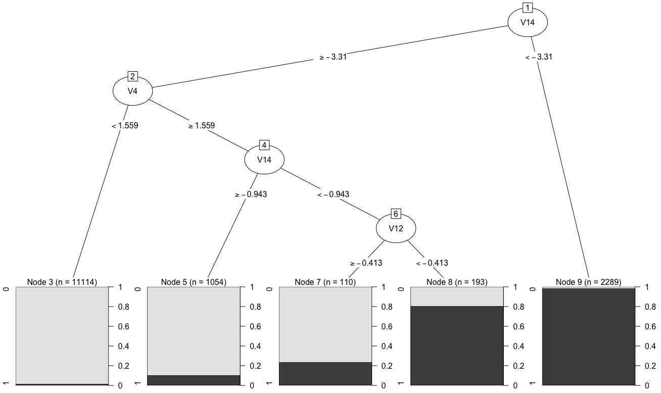
library(rpart)
model2 = rpart(Class ~ ., data = train_oversampled)

tree2

## 테스트 세트의 사기 확률 예측
scores2 = predict(model2, newdata = test, type = "prob")[, 2]

## 테스트 세트의 클래스(사기/정상) 예측
predicted_class2 = factor(ifelse(scores2 > 0.5, 1, 0))

## 혼동 행렬 & 정확도
library(caret)
CM2 = confusionMatrix(data = predicted_class2, reference = test$Class)

          Reference
Prediction     0     1
         0 11967    34
         1    87   212       Accuracy : 0.9901626

library(pROC)
auc(roc(response = test$Class, predictor = scores2)) ## ROC 곡선 하의 면적(AUC)

Area under the curve: 0.9538

탐지 모델 배포 비용

알고리즘 평가 시 서로 다른 사기 탐지 비용을 고려
비용은 다음에 연관됨
- 오분류 오류(거짓 양성·거짓 음성)와
- 정분류(진양성·진음성)

비용 행렬

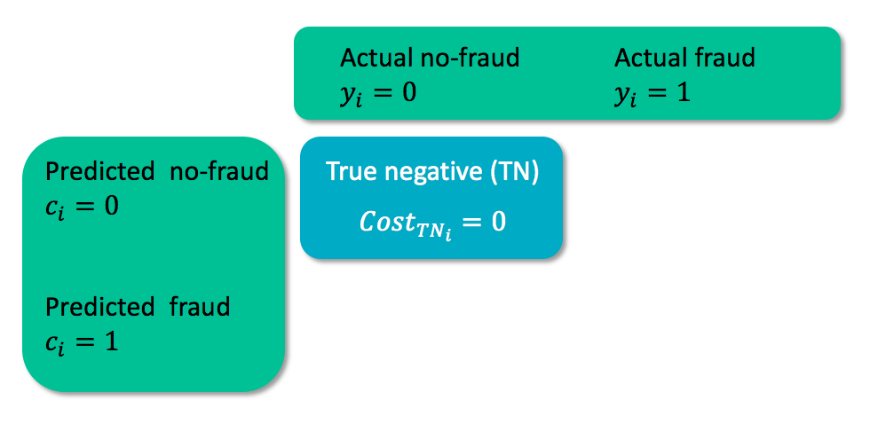
cost_matrix_1

$y_i$ = 사례 $i$의 실제 클래스
$c_i$ = 사례 $i$의 예측 클래스

비용 행렬

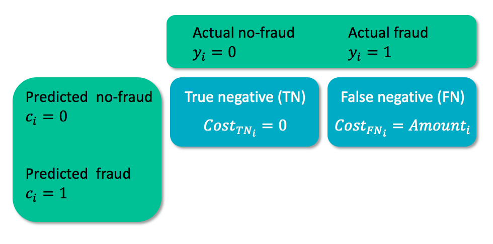
cost_matrix_2

$y_i$ = 사례 $i$의 실제 클래스
$c_i$ = 사례 $i$의 예측 클래스

비용 행렬

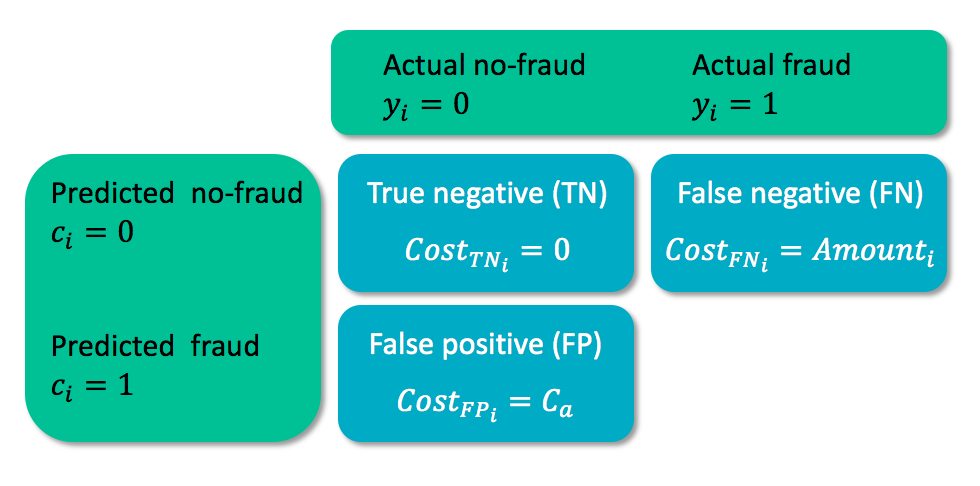
cost_matrix_3

$C_a$ = 사례 분석 비용

비용 행렬

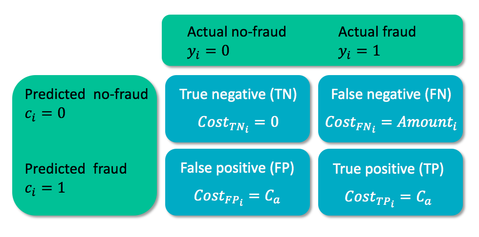
cost_matrix_4

$C_a$ = 사례 분석 비용

탐지 모델의 비용 지표

각 사례의 실제 비용을 반영: $$Cost(model)=\sum_{i=1}^{N}y_i(1-c_i)Amount_i + c_iC_a$$
- $y_i$ = 사례 $i$의 실제 클래스
- $c_i$ = 사례 $i$의 예측 클래스

cost_model = function(predicted.classes, true.classes, amounts, fixedcost) {

    cost = sum(true.classes * (1 - predicted.classes) * amounts +
               predicted.classes * fixedcost)

    return(cost)
}

사기 탐지의 실제 비용

## SMOTE 미사용 시 총비용:
cost_model(predicted_class1, test$Class, test$Amount, fixedcost = 10)

10061.8

## SMOTE 사용 시 총비용:
cost_model(predicted_class2, test$Class, test$Amount, fixedcost = 10)

7431.93

손실이 26% 감소합니다!

Ayo berlatih!

R로 배우는 사기 탐지