가우시안 분포

R로 배우는 Mixture Models

Victor Medina

Researcher at The University of Edinburgh

성별 데이터셋에 혼합 모델 적용

혼합 모델 적합 패키지

mixtools
- 포아송 분포가 구현되어 있지 않음.
bayesmix
- 베이지안 추론은 본 강의 범위를 벗어남.
EMCluster
- 가우시안 분포만 지원.
flexmix
- 필요한 모든 분포를 지원하며 복잡한 모델 구현 가능.

가우시안 분포의 특성

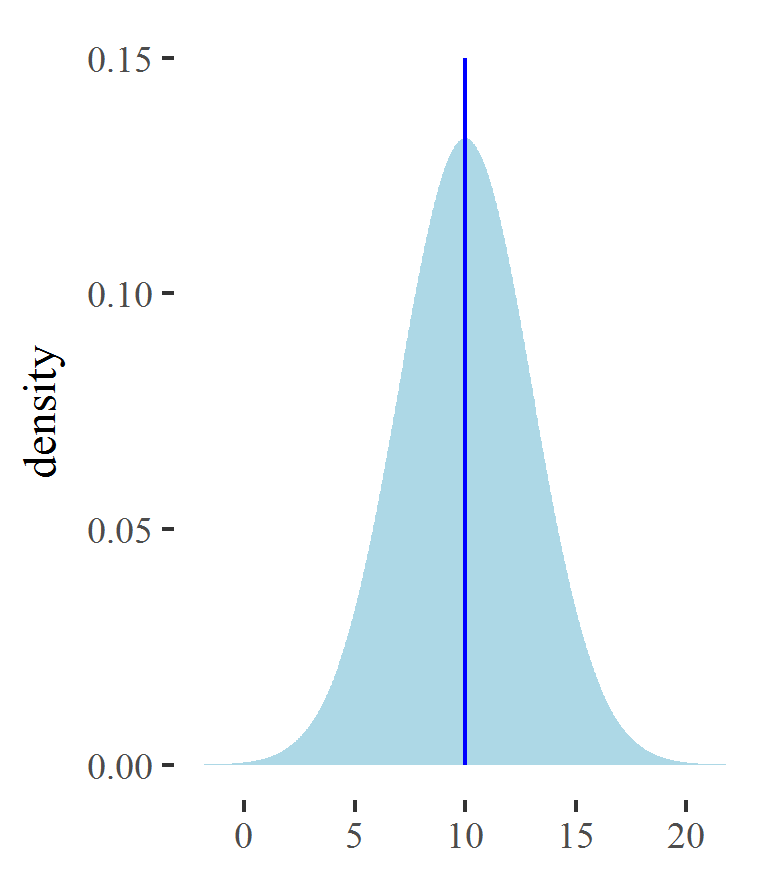
평균

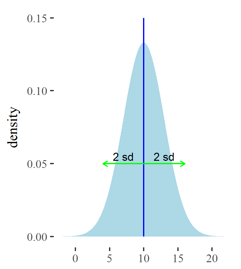
표준편차

가우시안 분포에서 표본 추출

가우시안 분포에서 표본 생성:

rnorm(n, mean, sd)

예시: 평균 10, 표준편차 5인 가우시안 분포에서 100개의 값 생성

> population_sample <- rnorm(n = 100, mean = 10, sd = 5)
> head(population_sample)

[1]  6.248874  9.564190 16.006521  9.139647 10.114969 16.423538

평균 추정

평균과 표준편차를 모르고 관측값만 알고 있음
- 관측값으로부터 추정해야 함
평균 추정에는 표본 평균을 계산

> mean_estimate <- mean(population_sample)

10.35759

sd 추정 절차

$$value_i\rightarrow (. -mean\_estimate)\rightarrow (.)^2\rightarrow mean (.)\rightarrow \sqrt{(.)}$$

> population_sample %>%  
+   subtract(mean_estimate) %>%
+   raise_to_power(2) %>% mean() %>% sqrt()

5.318641

sd 함수 사용

> standard_deviation_estimate <- sd(population_sample)
> standard_deviation_estimate

5.345435

추정된 가우시안 분포 시각화

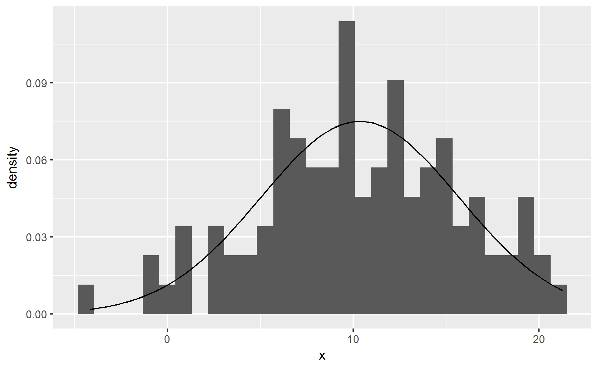
# Transform the sample into a data frame
population_sample <- data.frame(x = population_sample)

# Plot the histogram
ggplot(data = population_sample) + 
   geom_histogram(aes(x = x, y = ..density..)) +
   stat_function(geom = "line", 
                 fun = dnorm, 
                 args = list(mean = mean_estimate, 
                             sd = standard_deviation_estimate))

연습해 봅시다!

R로 배우는 Mixture Models