導関数でモデルパラメータを更新する

PyTorchで学ぶIntroduction to Deep Learning

Jasmin Ludolf

Senior Data Science Content Developer, DataCamp

導関数のたとえ

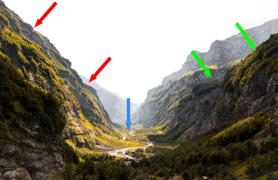
導関数は「曲線の傾き」を表す

傾きが急（赤矢印）：
- ステップが大、導関数は大
傾きが緩（緑矢印）：
- ステップが小、導関数は小
谷底（青矢印）：
- 平坦、導関数は0

谷の画像

凸関数と非凸関数

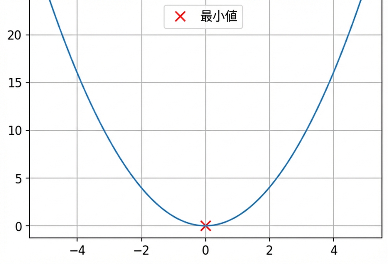
これは凸関数です

凸関数の例

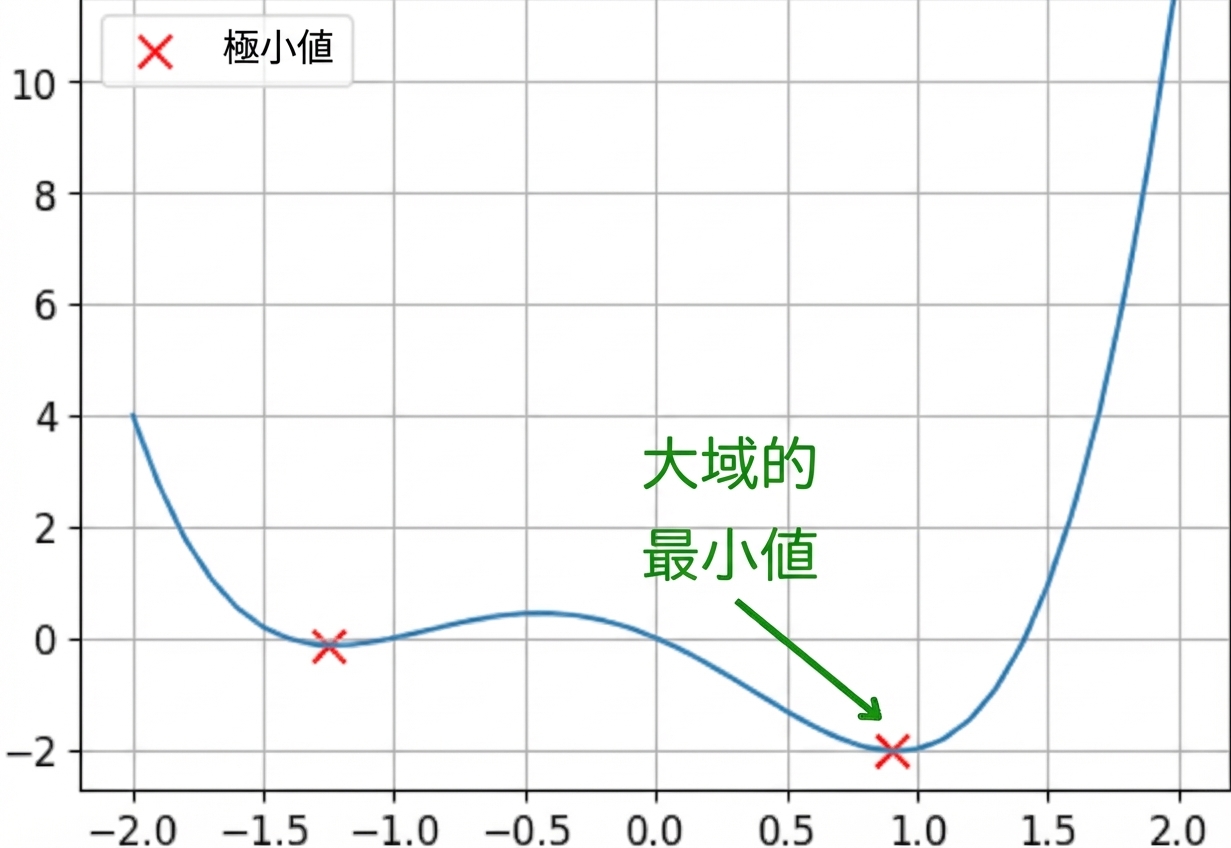
これは非凸関数です

大域的最小値を示した非凸関数の例

導関数と学習のつながり

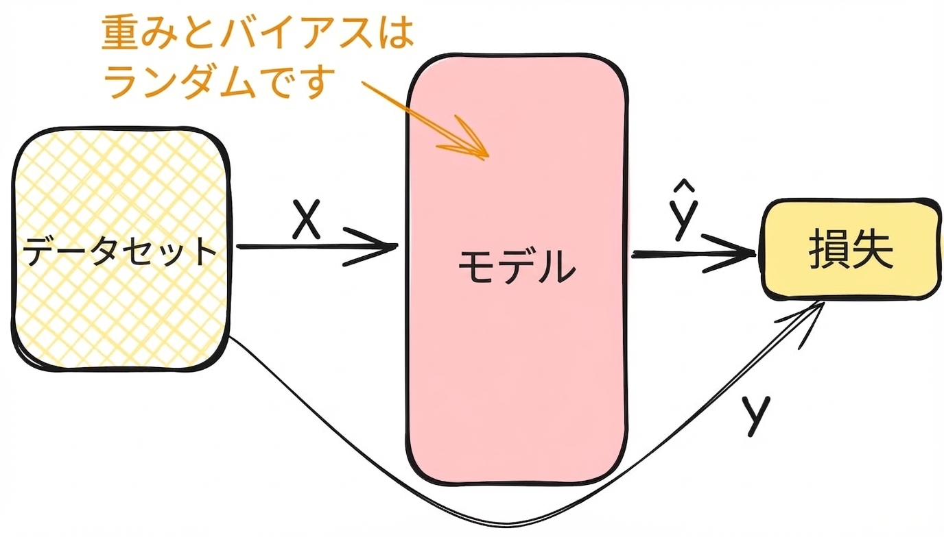
学習時の順伝播で損失を計算

$$ 損失の計算

導関数と学習のつながり

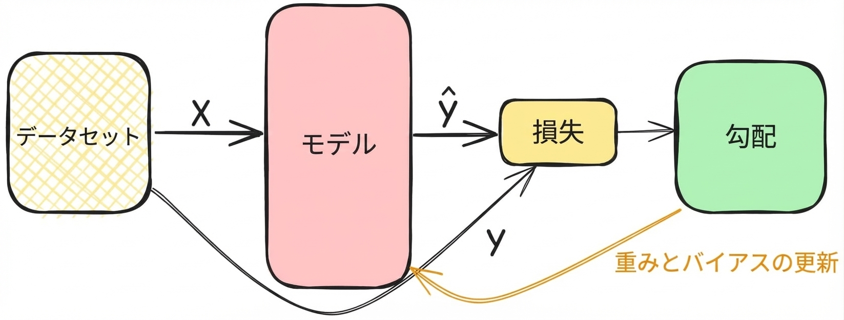
勾配で損失を最小化し、層の重みとバイアスを調整
層が調整されるまで反復

$$ 勾配の計算

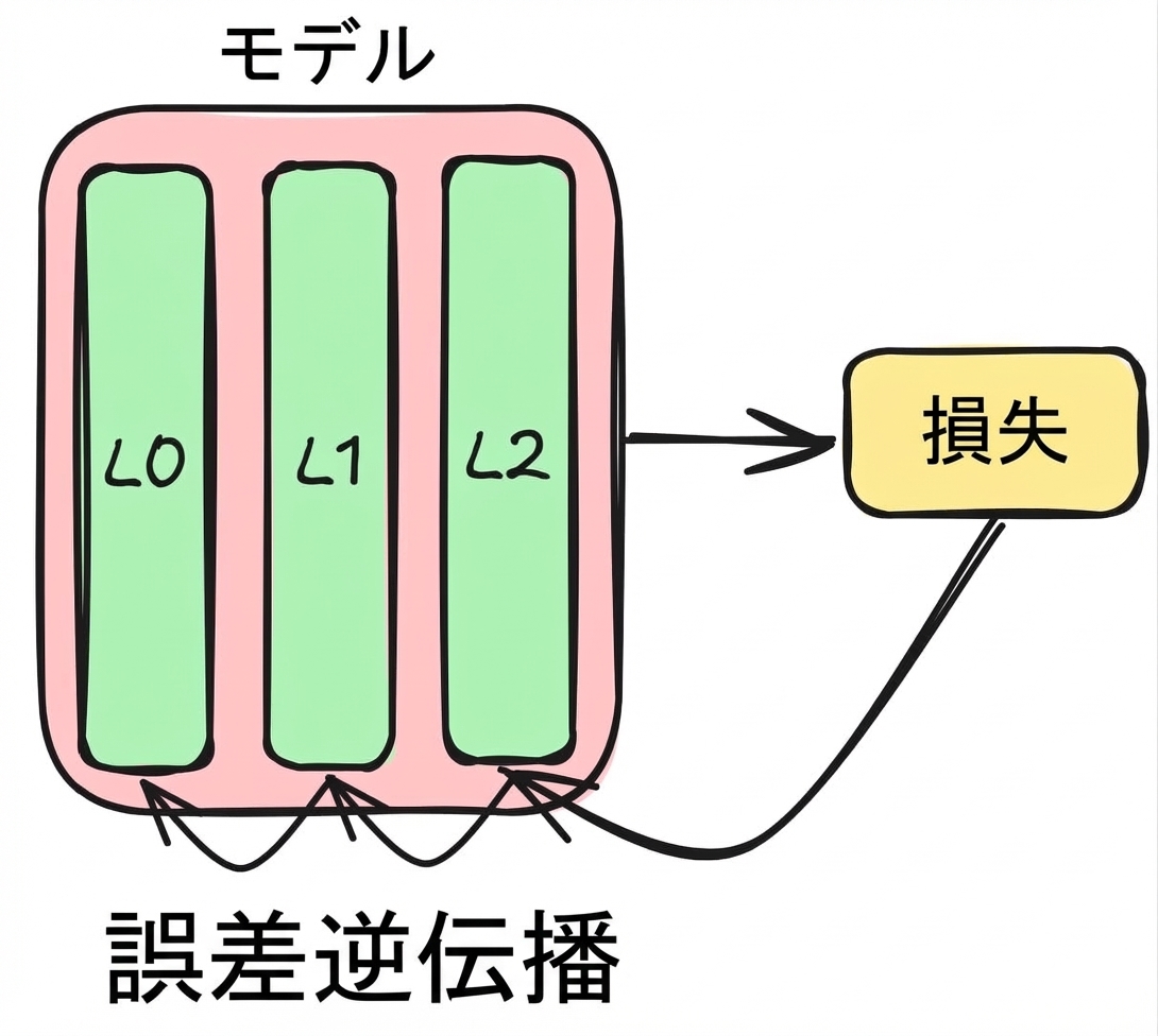
誤差逆伝播の基礎

3層のネットワークを考える:
- まず $L2$ の損失勾配から始める
- $L2$ から $L1$ の勾配を計算
- すべての層に繰り返す（$L1$, $L0$）

誤差逆伝播の図

PyTorchでの誤差逆伝播

# Run a forward pass 
model = nn.Sequential(nn.Linear(16, 8),
                      nn.Linear(8, 4),
                      nn.Linear(4, 2))
prediction = model(sample)


# Calculate the loss and gradients
criterion = CrossEntropyLoss()
loss = criterion(prediction, target)
loss.backward()

# Access each layer's gradients
model[0].weight.grad
model[0].bias.grad
model[1].weight.grad
model[1].bias.grad
model[2].weight.grad
model[2].bias.grad

手動でモデルパラメータを更新

# Learning rate is typically small
lr = 0.001

# Update the weights
weight = model[0].weight
weight_grad = model[0].weight.grad


weight = weight - lr * weight_grad


# Update the biases
bias = model[0].bias
bias_grad = model[0].bias.grad

bias = bias - lr * bias_grad

各層の勾配にアクセス
学習率を掛ける
その積を重みに引く

勾配降下法

非凸関数には勾配降下法を用いる
PyTorch では オプティマイザで簡略化
- 確率的勾配降下法（SGD）

import torch.optim as optim

# Create the optimizer
optimizer = optim.SGD(model.parameters(), lr=0.001)


# Perform parameter updates
optimizer.step()

練習しましょう！

PyTorchで学ぶIntroduction to Deep Learning