折れ線グラフ入門

Seaborn を使ったデータ可視化入門

Content Team

DataCamp

ラインプロットとは？

2種類のリレーショナルプロット：散布図と折れ線グラフ

散布図
各点は独立した観測を表す

折れ線グラフ

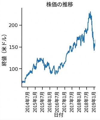
各点は同じ「対象」を表し、通常は時間の経過に沿って追跡される

Line plot of stock price over time

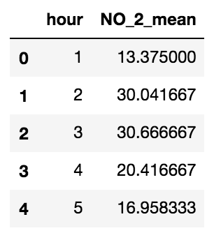
大気汚染データ

市内各所に設置された大気測定ステーション
二酸化窒素濃度を測定した大気サンプル

First five rows of air pollution DataFrame

散布図

import matplotlib.pyplot as plt
import seaborn as sns

sns.relplot(x="hour", y="NO_2_mean", 
            data=air_df_mean, 
            kind="scatter")

plt.show()

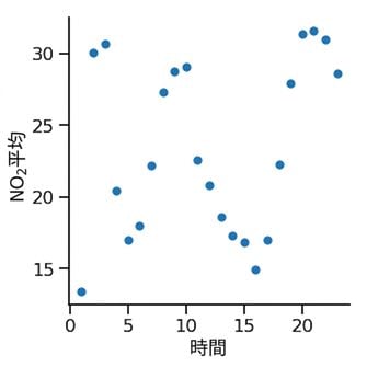
Scatter plot of average nitrogen dioxide over time

折れ線グラフ

import matplotlib.pyplot as plt
import seaborn as sns

sns.relplot(x="hour", y="NO_2_mean", 
            data=air_df_mean, 
            kind="line")

plt.show()

Line plot of average nitrogen dioxide over time

場所によるサブグループ分け

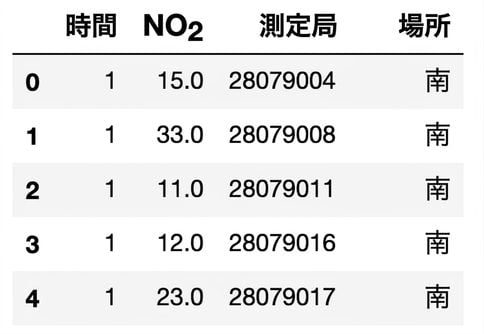
First five rows of air pollution by location DataFrame

場所によるサブグループ分け

import matplotlib.pyplot as plt
import seaborn as sns

sns.relplot(x="hour", y="NO_2_mean", 
            data=air_df_loc_mean, 
            kind="line",
            style="location", 
            hue="location")

plt.show()

Line plot of average nitrogen dioxide over time per region

マーカーを追加する

import matplotlib.pyplot as plt
import seaborn as sns

sns.relplot(x="hour", y="NO_2_mean", 
            data=air_df_loc_mean, 
            kind="line", 
            style="location", 
            hue="location",
            markers=True)

plt.show()

Line plot with markers added

線のスタイルによる区別をオフにする

import matplotlib.pyplot as plt
import seaborn as sns

sns.relplot(x="hour", y="NO_2_mean", 
            data=air_df_loc_mean, 
            kind="line", 
            style="location", 
            hue="location",
            markers=True,
            dashes=False)

plt.show()

Line plot with markers and solid lines

各x値に複数の観測値

First five rows of air pollution DataFrame per station

各x値に複数の観測値

散布図

import matplotlib.pyplot as plt
import seaborn as sns

sns.relplot(x="hour", y="NO_2", 
            data=air_df, 
            kind="scatter")

plt.show()

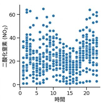
Scatter plot of nitrogen dioxide for all stations over time

各x値に複数の観測値

折れ線グラフ

import matplotlib.pyplot as plt
import seaborn as sns

sns.relplot(x="hour", y="NO_2", 
            data=air_df, 
            kind="line")

plt.show()

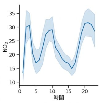
Line plot of nitrogen dioxide for all stations over time

各x値に複数の観測値

網掛け部分は信頼区間を示す

データセットが無作為標本であると仮定する
平均値がこの区間内にあると95%の信頼をもって言える
推定値の不確実性を示す

Line plot of nitrogen dioxide for all stations over time

信頼区間を標準偏差に置き換える

import matplotlib.pyplot as plt
import seaborn as sns

sns.relplot(x="hour", y="NO_2", 
            data=air_df, 
            kind="line",
            errorbar="sd")

plt.show()

Line plot with standard deviation

信頼区間を非表示にする

import matplotlib.pyplot as plt
import seaborn as sns

sns.relplot(x="hour", y="NO_2", 
            data=air_df, 
            kind="line",
            errorbar=None)

plt.show()

Line plot with no confidence interval

練習しましょう！

Seaborn を使ったデータ可視化入門