代表値

Rで学ぶ統計入門

Maggie Matsui

Content Developer, DataCamp

哺乳類の睡眠データ

msleep

# A tibble: 83 x 11
   name             genus       vore  order        sleep_total sleep_rem sleep_cycle awake
   <chr>            <chr>       <chr> <chr>              <dbl>     <dbl>       <dbl> <dbl>
 1 Cheetah          Acinonyx    carni Carnivora           12.1      NA         NA     11.9
 2 Owl monkey       Aotus       omni  Primates            17         1.8       NA      7 
 3 Mountain beaver  Aplodontia  herbi Rodentia            14.4       2.4       NA      9.6
 4 Greater short... Blarina     omni  Soricomorpha        14.9       2.3       0.133   9.1 
 5 Cow              Bos         herbi Artiodactyla         4         0.7       0.667  20  
 6 Three-toed sloth Bradypus    herbi Pilosa              14.4       2.2       0.767   9.6 
 7 Northern fur...  Callorhinus carni Carnivora            8.7       1.4       0.383  15.3 
# ... with 76 more rows, and 2 more variables: brainwt <dbl>, bodywt <dbl>

ヒストグラム

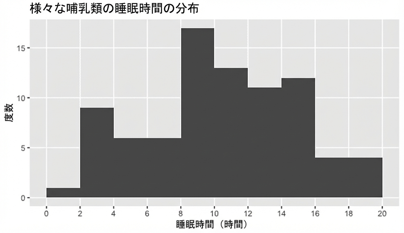
哺乳類の睡眠時間のヒストグラム

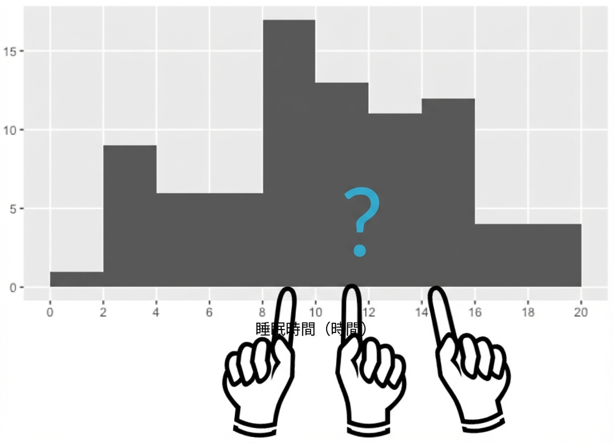
このデータの哺乳類は通常どれくらい眠るか

一般的な値は？

データの中心はどこか？

平均
中央値
最頻値

クエスチョンマークと指差しのあるヒストグラム

代表値：平均

  name                       sleep_total
1 Cheetah                           12.1
2 Owl monkey                        17.0 
3 Mountain beaver                   14.4
4 Greater short-tailed shrew        14.9
...

$$\text{平均睡眠時間}=\frac{12.1 + 17.0 + 14.4 + 14.9 + ...}{83} = 10.43$$

mean(msleep$sleep_total)

10.43373

代表値：中央値

sort(msleep$sleep_total)

 [1]  1.9  2.7  2.9  3.0  3.1  3.3  3.5  3.8  3.9  4.0  4.4  5.2  5.3  5.3  5.4  5.6  6.2
...
[52] 11.5 12.1 12.5 12.5 12.5 12.5 12.8 12.8 13.0 13.5 13.7 13.8 14.2 14.3 14.4 14.4 14.5
[69] 14.6 14.9 14.9 15.6 15.8 15.8 15.9 16.6 17.0 17.4 18.0 18.1 19.4 19.7 19.9

sort(msleep$sleep_total)[42]

10.1

median(msleep$sleep_total)

10.1

代表値：最頻値

最頻値

# 'sleep_total' を降順で集計
msleep %>% count(sleep_total, sort = TRUE)

   sleep_total     n
         <dbl> <int>
 1        12.5     4
 2        10.1     3
 3         5.3     2
 4         6.3     2
 ...

# 'vore' を降順で集計
msleep %>% count(vore, sort = TRUE)

  vore        n
  <chr>   <int>
1 herbi      32
2 omni       20
3 carni      19
4 NA          7
5 insecti     5

食性が昆虫食のデータの抽出

msleep %>% 
  filter(vore == "insecti")

  name                  genus        vore    order        sleep_total
  <chr>                 <chr>        <chr>   <chr>              <dbl>
1 Big brown bat         Eptesicus    insecti Chiroptera          19.7
2 Little brown bat      Myotis       insecti Chiroptera          19.9
3 Giant armadillo       Priodontes   insecti Cingulata           18.1
4 Eastern american mole Scalopus     insecti Soricomorpha         8.4

昆虫食の睡眠統計の要約

msleep %>% 
  filter(vore == "insecti") %>%

  summarize(mean_sleep = mean(sleep_total),
           median_sleep = median(sleep_total))

  mean_sleep median_sleep
       <dbl>        <dbl> 
1      16.52         18.9

外れ値の追加

msleep %>% 
  filter(vore == "insecti")

  name                  genus        vore    order        sleep_total
  <chr>                 <chr>        <chr>   <chr>              <dbl>
1 Big brown bat         Eptesicus    insecti Chiroptera          19.7
2 Little brown bat      Myotis       insecti Chiroptera          19.9
3 Giant armadillo       Priodontes   insecti Cingulata           18.1
4 Eastern american mole Scalopus     insecti Soricomorpha         8.4
5 Mystery insectivore   ...          ...     ...                  0.0

外れ値追加後の要約統計

msleep %>% 
  filter(vore == "insecti") %>%

  summarize(mean_sleep = mean(sleep_total),
           median_sleep = median(sleep_total))

  mean_sleep median_sleep
       <dbl>        <dbl>
1      13.22         18.1

平均: 16.5 → 13.2

中央値: 18.9 → 18.1

どの指標を使うべきか

# 昆虫食のヒストグラムを作成
msleep %>% 
  filter(vore == "insecti") %>%
  ggplot(aes(insecti)) +
    geom_histogram()

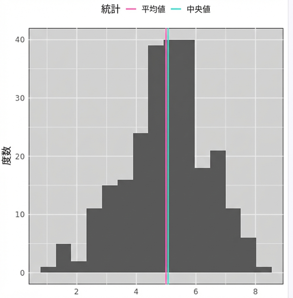
釣鐘型のヒストグラム。中央で赤と青の線が近接。赤=平均、青=中央値。

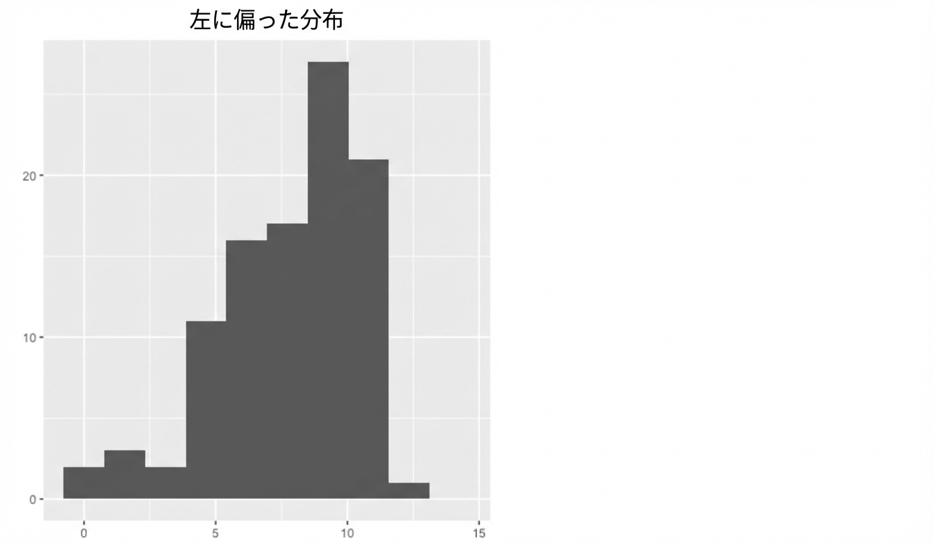
歪度

左側が少なく右側ほど多い分布のヒストグラム

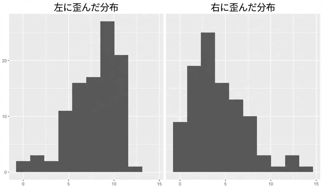
歪度

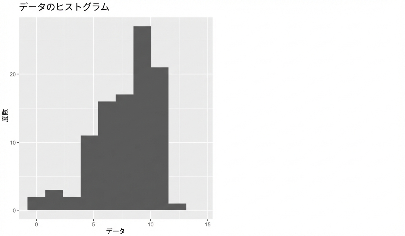
左裾が長く右に向かって増えるヒストグラム（左に歪んだ）

歪度

左側に多く右側が少ないヒストグラム（右に歪んだ）

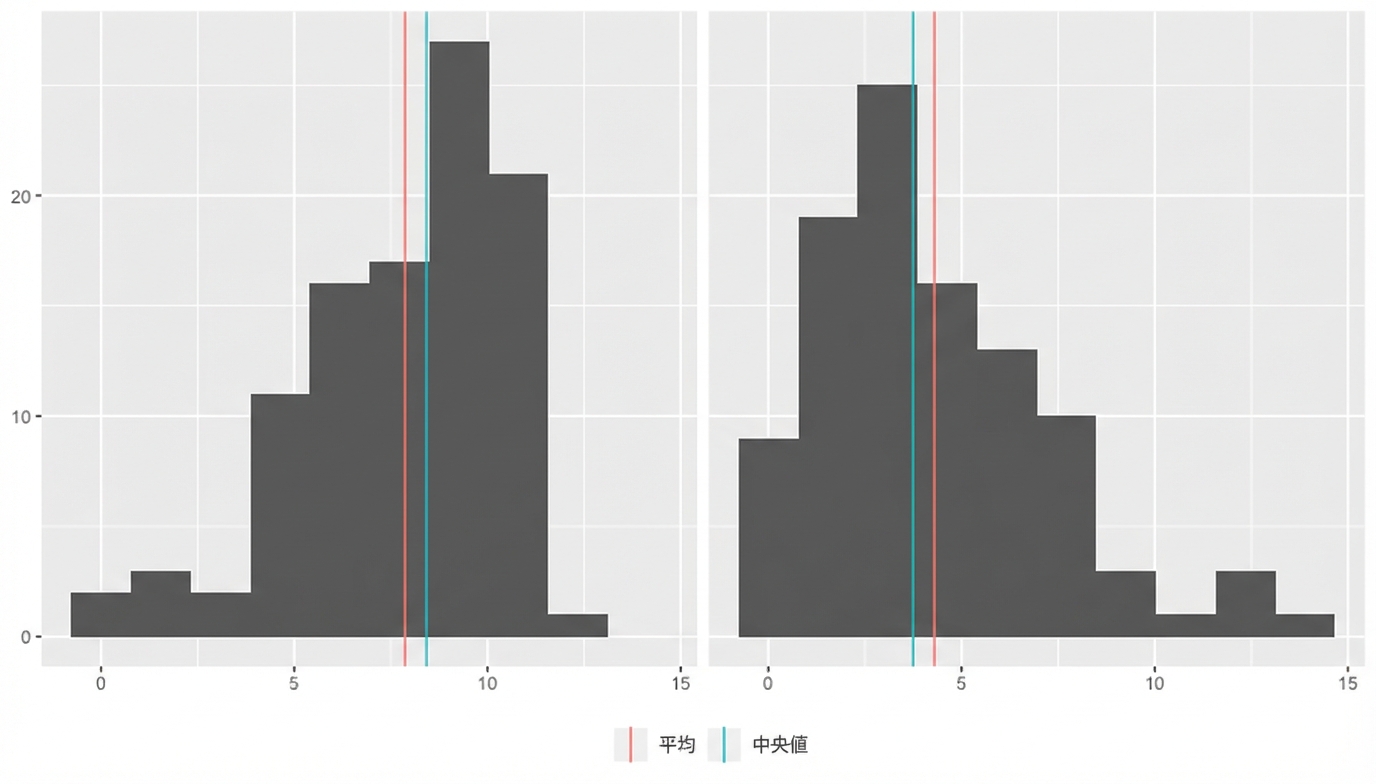
どの指標を使うべきか

前スライドと同じヒストグラム。平均（赤）と中央値（青）の線。左に歪んだ分布では平均<中央値。右に歪んだ分布では平均>中央値。

Passons à la pratique !

Rで学ぶ統計入門