中心極限定理

Rで学ぶ統計入門

Maggie Matsui

Content Developer, DataCamp

サイコロを5回振る

die <- c(1, 2, 3, 4, 5, 6)

# Roll 5 times sample_of_5 <- sample(die, 5, replace = TRUE) sample_of_5
1 3 4 1 1
mean(sample_of_5)
2.0


六面体のサイコロ

Rで学ぶ統計入門

サイコロを5回振る

# Roll 5 times and take mean
sample(die, 5, replace = TRUE) %>% mean()
4.4
sample(die, 5, replace = TRUE) %>% mean()
3.8
Rで学ぶ統計入門

サイコロを5回、10セット振る

10回繰り返す:

  • 5回振る
  • 平均を取る


sample_means <- replicate(10, sample(die, 5, replace = TRUE) %>% mean())

sample_means
3.8 4.0 3.8 3.6 3.2 4.8 2.6 3.0 2.6 2.0
Rで学ぶ統計入門

標本分布

標本平均の標本分布

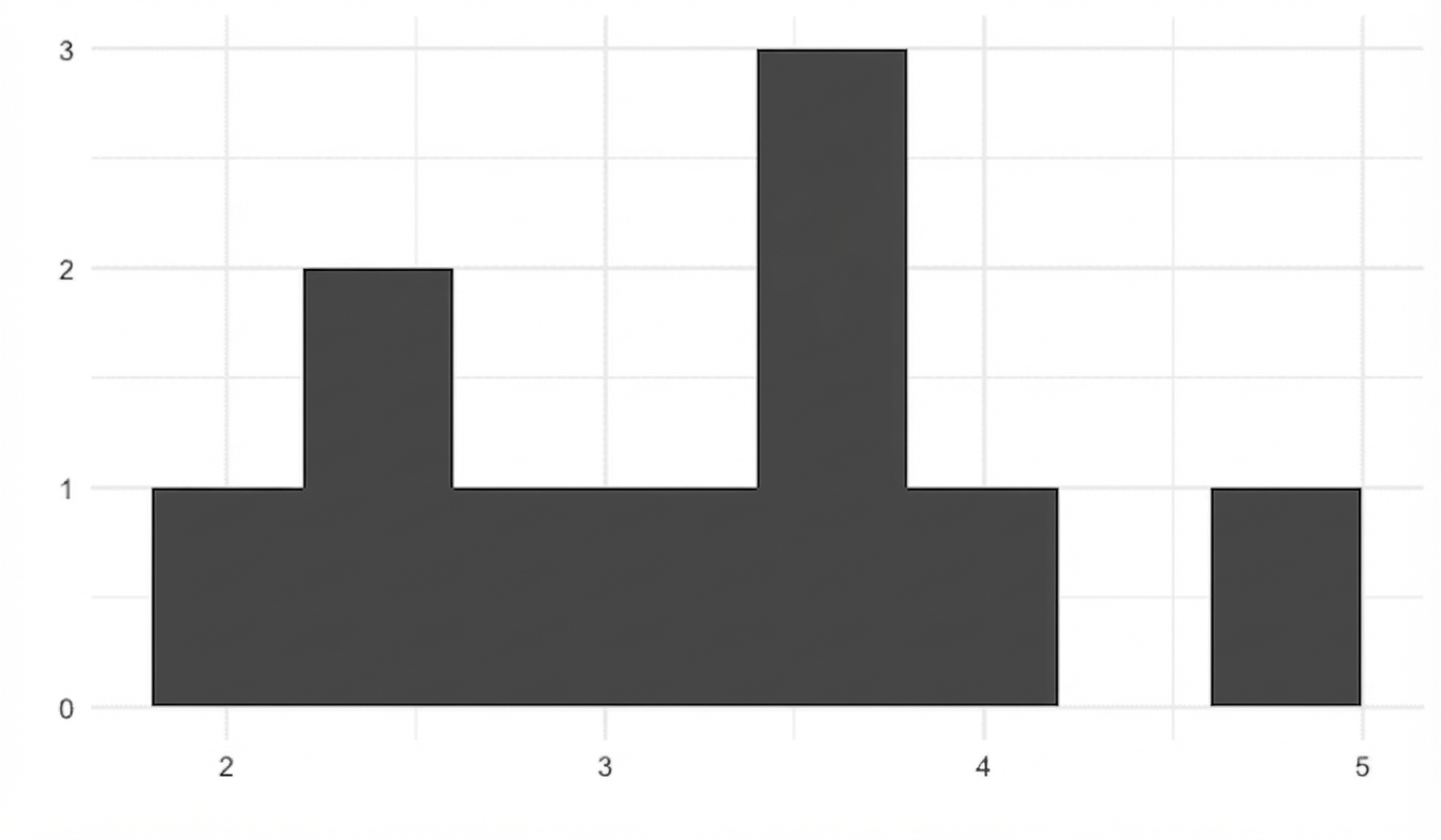
10個の標本平均のヒストグラム

Rで学ぶ統計入門

100個の標本平均

replicate(100, sample(die, 5, replace = TRUE) %>% mean())
2.8 3.2 1.8 4.6 4.0 2.8 4.4 2.4 3.4 2.8 4.2 3.4 ... 2.2 3.8 3.6 3.8 4.4 4.8 2.4
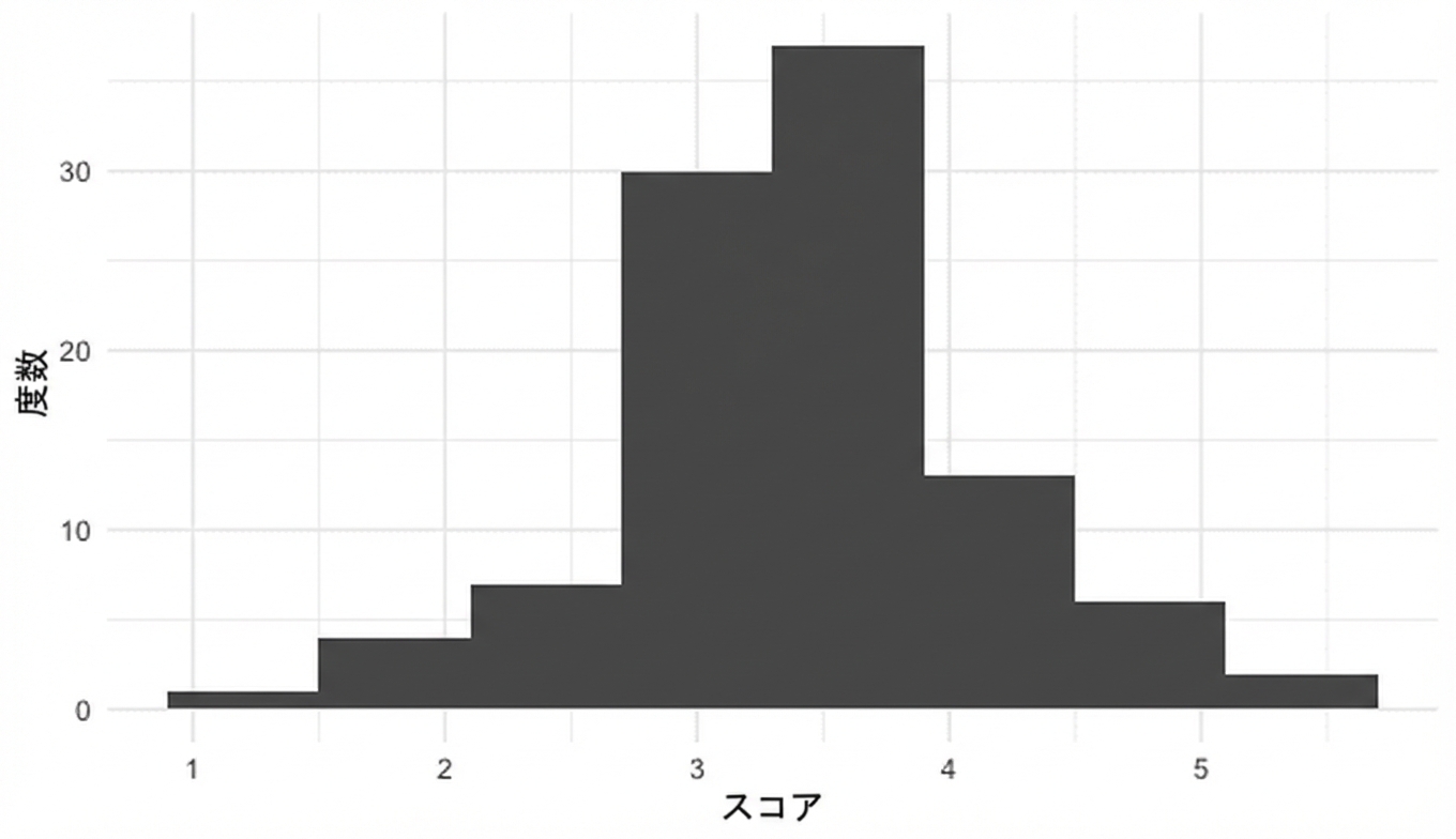
100個の標本平均のヒストグラム

Rで学ぶ統計入門

1000個の標本平均

sample_means <- replicate(1000, sample(die, 5, replace = TRUE) %>% mean())
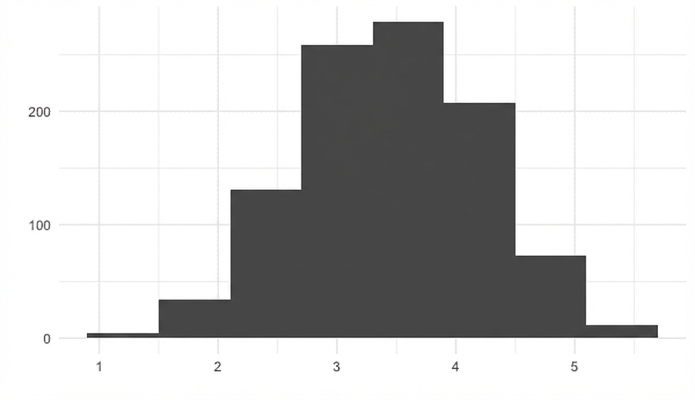
1000個の標本平均のヒストグラム

Rで学ぶ統計入門

中心極限定理

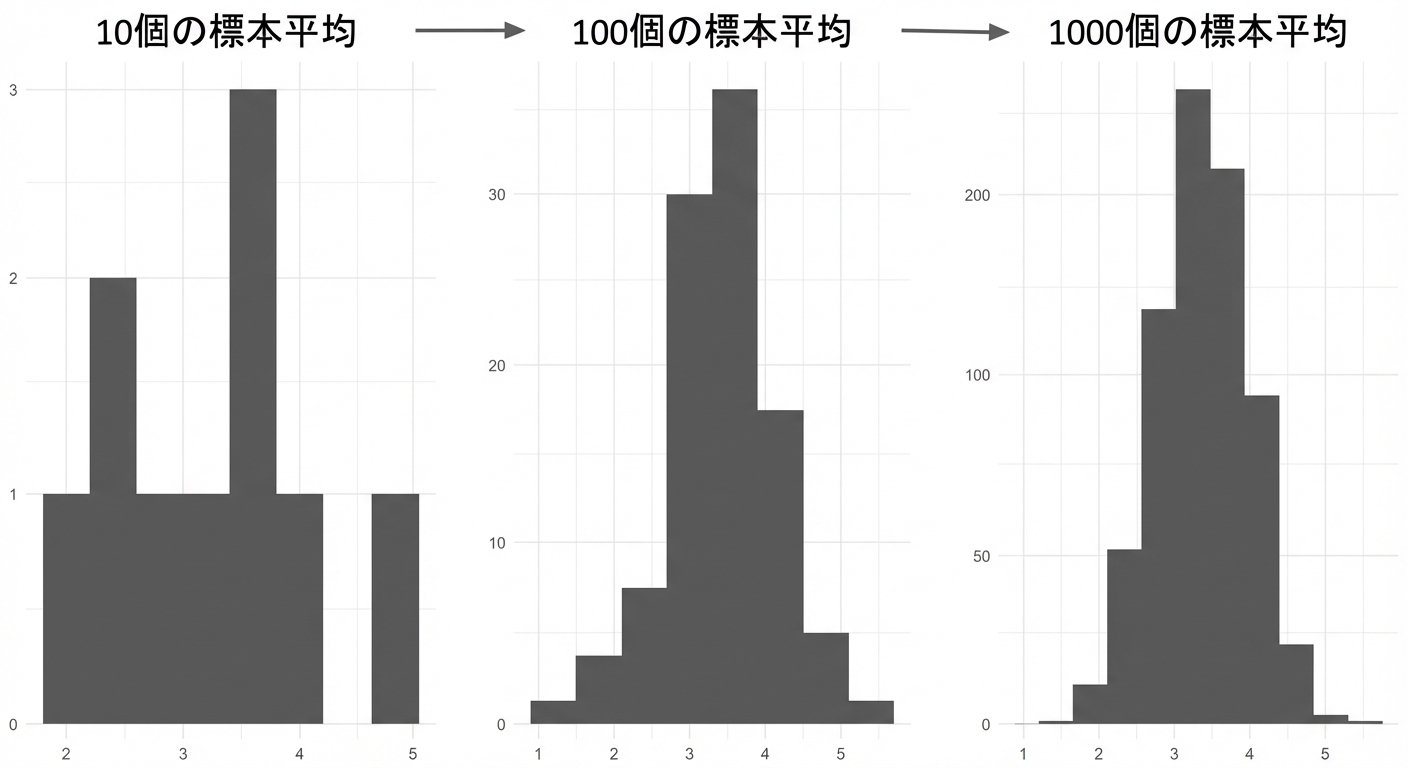
試行回数が増えるほど、統計量の標本分布は正規分布に近づく。

10・100・1000個の標本平均のヒストグラム(数が多いほど釣り鐘型に近づく)


* 標本はランダムかつ独立であること

Rで学ぶ統計入門

標準偏差とCLT

replicate(1000, sample(die, 5, replace = TRUE) %>% sd())
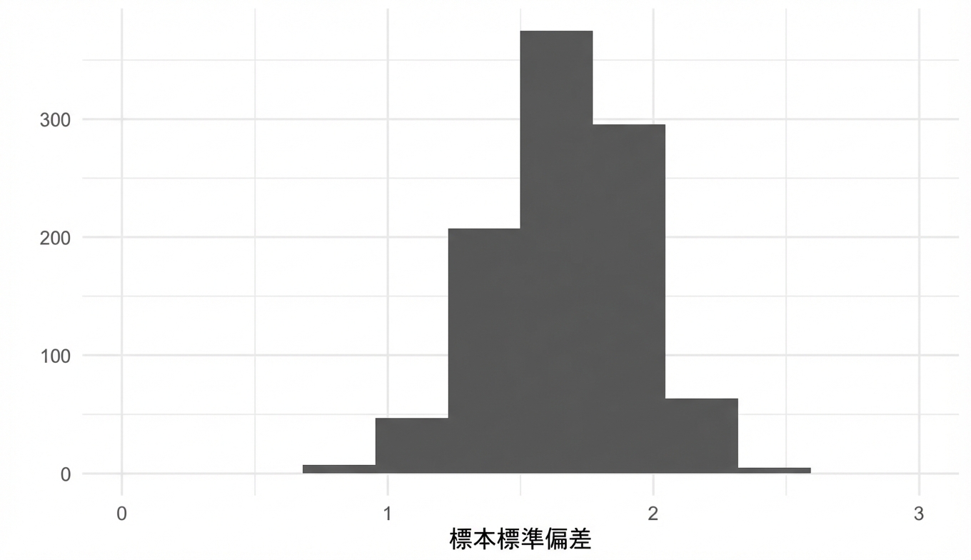
サイコロ5回の標準偏差1000個の分布

Rで学ぶ統計入門

割合とCLT

sales_team <- c("Amir", "Brian", "Claire", "Damian")

sample(sales_team, 10, replace = TRUE)
"Claire" "Brian"  "Brian"  "Brian"  "Damian" "Damian" "Brian"  "Brian" 
"Amir"   "Amir"
sample(sales_team, 10, replace = TRUE)
"Amir"   "Amir"   "Claire" "Amir"   "Amir"   "Brian"  "Amir"   "Claire" 
"Claire" "Claire"
Rで学ぶ統計入門

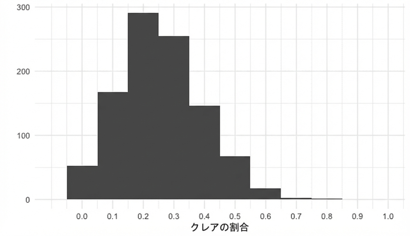
割合の標本分布

標本割合の分布も正規分布に近い

Rで学ぶ統計入門

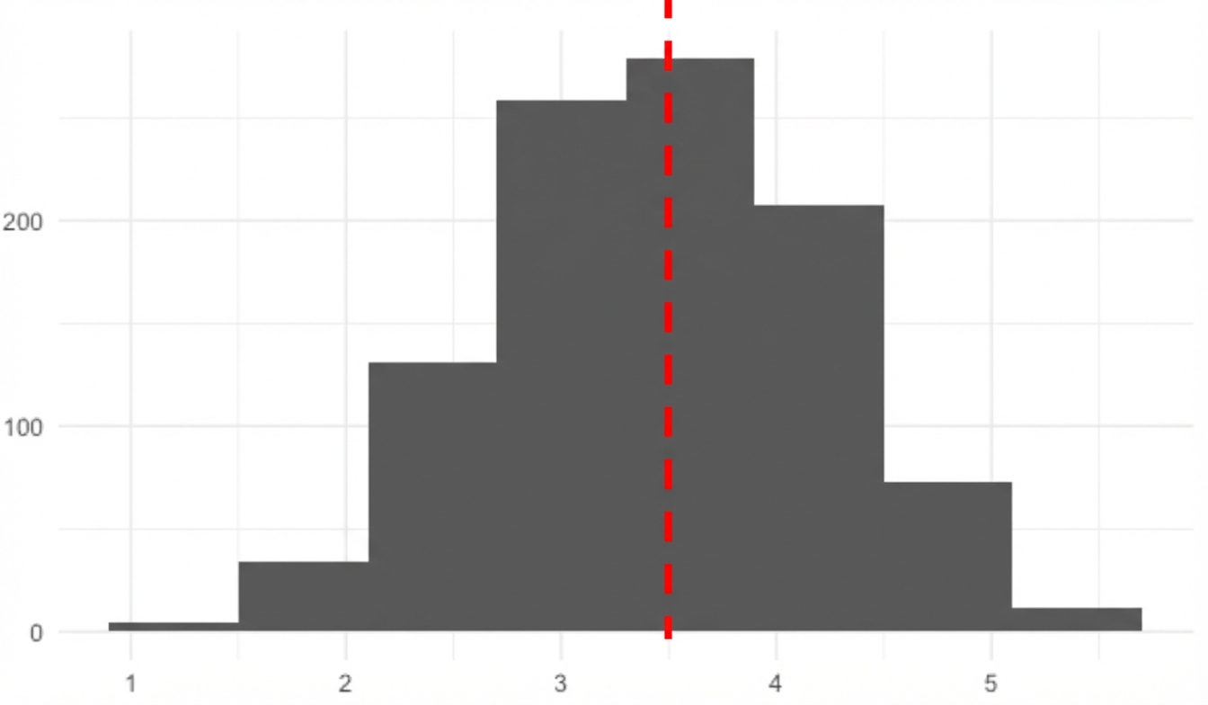
標本分布の平均

# Estimate expected value of die
mean(sample_means)
3.48
# Estimate proportion of "Claire"s
mean(sample_props)
0.26
  • 未知の母分布の特性を推定する

中央に破線のある標本平均の標本分布  

  • 大規模母集団の特性をより容易に推定する
Rで学ぶ統計入門

練習しましょう!

Rで学ぶ統計入門

Preparing Video For Download...