2変数の物語

Rで学ぶ回帰入門

Richie Cotton

Data Evangelist at DataCamp

スウェーデン自動車保険データ

各行はスウェーデンの1地域を表す。
63行ある。

n_claims	total_payment_sek
108	392.5
19	46.2
13	15.7
124	422.2
40	119.4
...	...

記述統計量

library(dplyr)
swedish_motor_insurance %>% 
  summarize_all(mean)

# A tibble: 1 x 2
  n_claims total_payment_sek
     <dbl>             <dbl>
1     22.9              98.2

swedish_motor_insurance %>% 
  summarize(
    correlation = cor(n_claims, total_payment_sek)
  )

# A tibble: 1 x 1
  correlation
        <dbl>
1       0.881

回帰とは？

応答変数と説明変数の関係を調べる統計モデル。
説明変数の値から、応答変数を予測できる。

n_claims	total_payment_sek
108	392.5
19	46.2
13	15.7
124	422.2
40	119.4
200	???

用語

応答変数（従属変数）

予測したい変数。

説明変数（独立変数）

応答変数の変化を説明する変数。

線形回帰とロジスティック回帰

線形回帰

応答変数は数値。

ロジスティック回帰

応答変数は論理値。

単回帰（線形／ロジスティック）

説明変数は1つだけ。

2変数の可視化

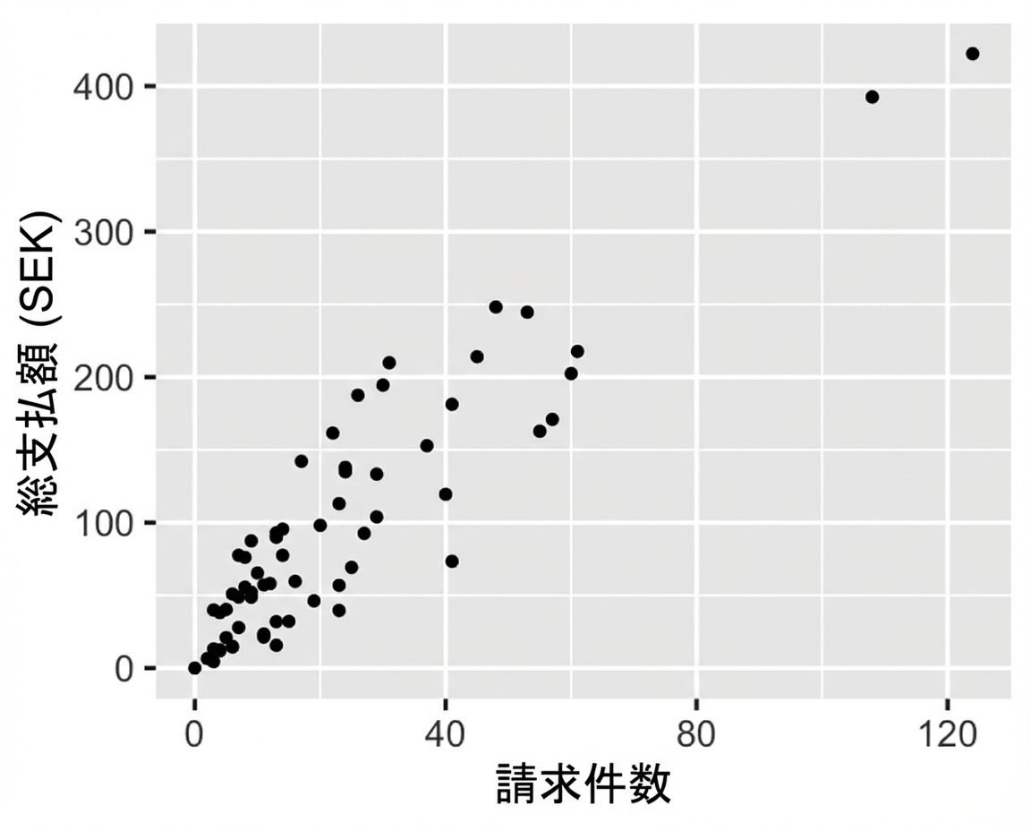
library(ggplot2)

ggplot(
  swedish_motor_insurance, 
  aes(n_claims, total_payment_sek)
) +
  geom_point()

総支払額と請求件数の散布図。請求件数が増えると支払額も増える。

線形トレンドラインの追加

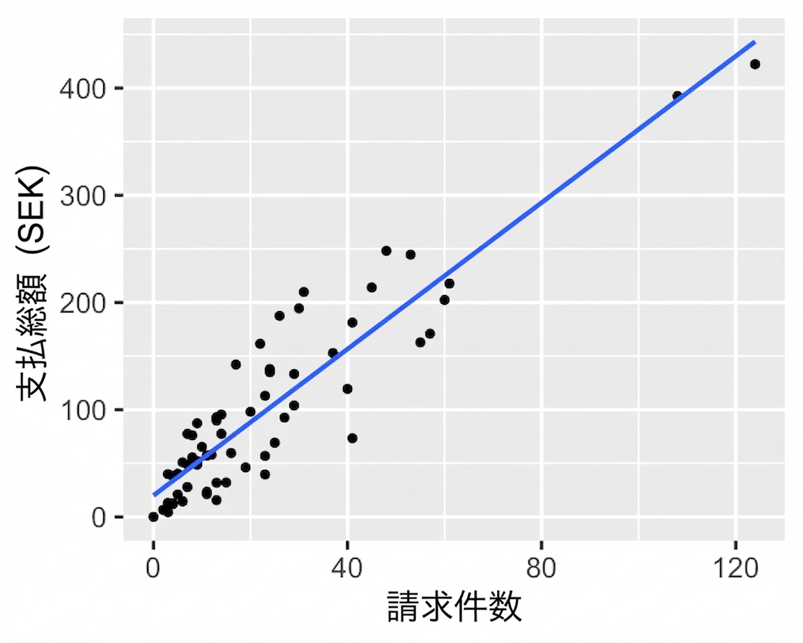
library(ggplot2)

ggplot(
  swedish_motor_insurance, 
  aes(n_claims, total_payment_sek)
) +
  geom_point() +
  geom_smooth(
    method = "lm", 
    se = FALSE
  )

先ほどの散布図に、線形回帰で求めたトレンドラインを追加。データに概ね適合している。

コースの流れ

第1章

線形回帰モデルの可視化と当てはめ。

第2章

線形回帰からの予測と係数の理解。

第3章

線形回帰モデルの良さの評価。

第4章

同様だがロジスティック回帰で実施。

練習しましょう！

Rで学ぶ回帰入門