ロジスティック回帰が必要な理由

Rで学ぶ回帰入門

Richie Cotton

Data Evangelist at DataCamp

銀行の解約データセット

has_churned	time_since_first_purchase	time_since_last_purchase
0	0.3993247	-0.5158691
1	-0.4297957	0.6780654
0	3.7383122	0.4082544
0	0.6032289	-0.6990435
...	...	...
応答	関係の長さ	直近活動

¹ https://www.rdocumentation.org/packages/bayesQR/topics/Churn

解約と直近度：線形モデル

mdl_churn_vs_recency_lm <- lm(has_churned ~ time_since_last_purchase, data = churn)

Call:
lm(formula = has_churned ~ time_since_last_purchase, data = churn)

Coefficients:
             (Intercept)  time_since_last_purchase  
                 0.49078                   0.06378

coeffs <- coefficients(mdl_churn_vs_recency_lm)
intercept <- coeffs[1]
slope <- coeffs[2]

線形モデルの可視化

ggplot(
  churn, 
  aes(time_since_last_purchase, has_churned)
) +
  geom_point() +
  geom_abline(intercept = intercept, slope = slope)

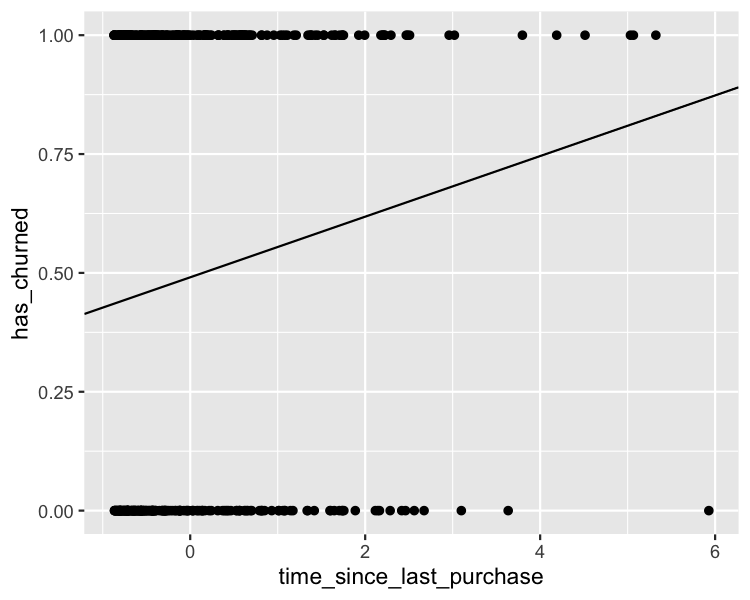
「予測」は解約の量ではなく、解約確率です。

顧客が解約したか否かと最終購入からの経過時間の散布図。点は y=0 または y=1 にのみある。線形トレンド線は、経過時間が長いほど解約確率が上がることを示す。

ズームアウト

ggplot(
  churn, 
  aes(days_since_last_purchase, has_churned)
) +
  geom_point() +
  geom_abline(intercept = intercept, slope = slope) +
  xlim(-10, 10) +
  ylim(-0.2, 1.2)

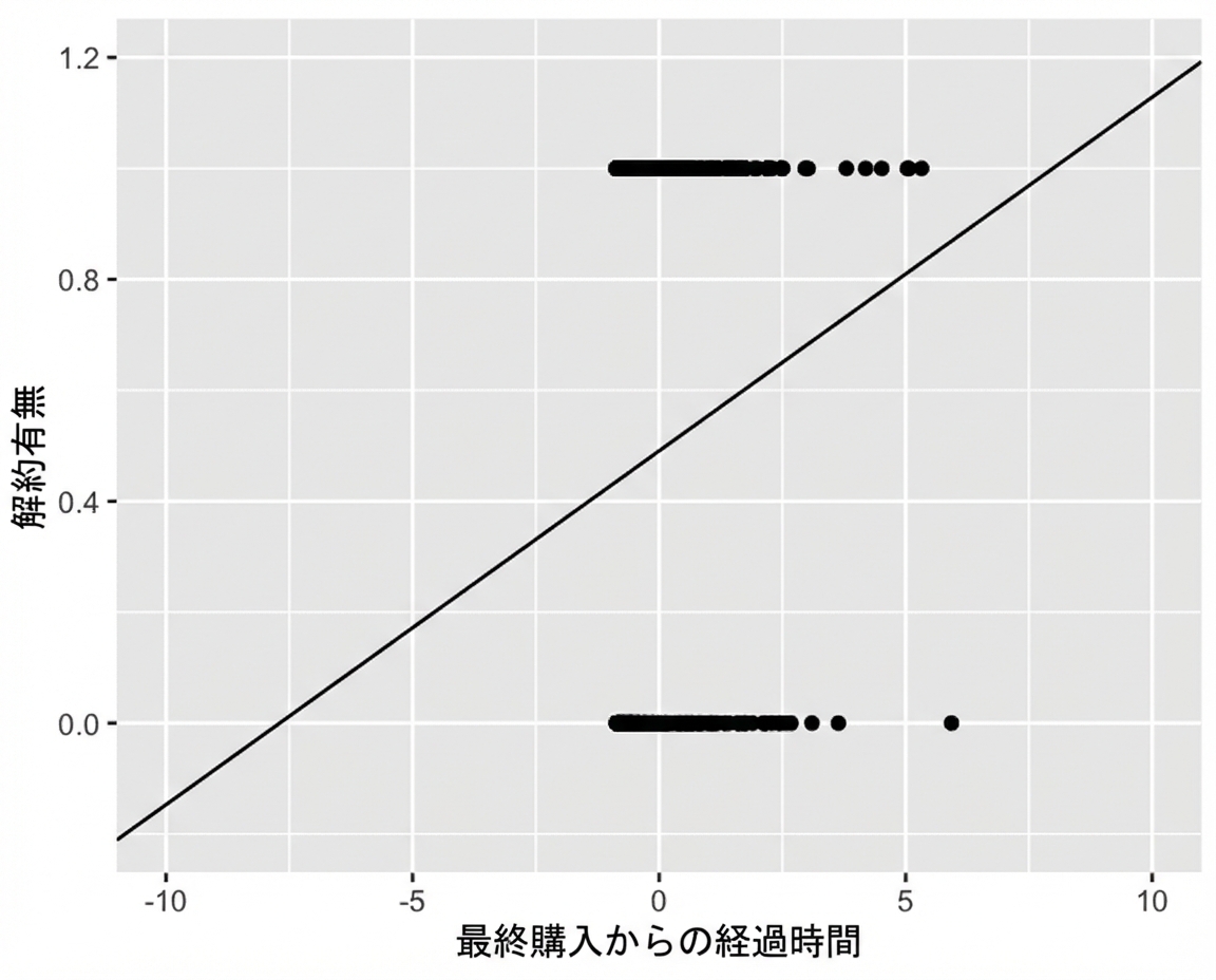
前図と同じ散布図。軸を広げると、線形のトレンド線が y=0 未満や y=1 超に伸び、確率の範囲を外れてしまうことがわかる。

ロジスティック回帰とは？

一般化線形モデルの一種。
応答変数が論理（真偽）のときに使用。
応答はロジスティック（S字）曲線に従う。

glm() による線形回帰

glm(has_churned ~ time_since_last_purchase, data = churn, family = gaussian)

Call:  glm(formula = has_churned ~ time_since_last_purchase, family = gaussian, 
    data = churn)

Coefficients:
             (Intercept)  time_since_last_purchase  
                 0.49078                   0.06378  

Degrees of Freedom: 399 Total (i.e. Null);  398 Residual
Null Deviance:        100 
Residual Deviance: 98.02     AIC: 578.7

ロジスティック回帰：binomial を指定した glm()

mdl_recency_glm <- glm(has_churned ~ time_since_last_purchase, data = churn, family = binomial)

Call:  glm(formula = has_churned ~ time_since_last_purchase, family = binomial, 
    data = churn)

Coefficients:
             (Intercept)  time_since_last_purchase  
                -0.03502                   0.26921  

Degrees of Freedom: 399 Total (i.e. Null);  398 Residual
Null Deviance:        554.5 
Residual Deviance: 546.4     AIC: 550.4

ロジスティックモデルの可視化

ggplot(
  churn, 
  aes(time_since_last_purchase, has_churned)
) +
  geom_point() +
  geom_abline(
    intercept = intercept, slope = slope
  ) +
  geom_smooth(
    method = "glm", 
    se = FALSE, 
    method.args = list(family = binomial)
  )

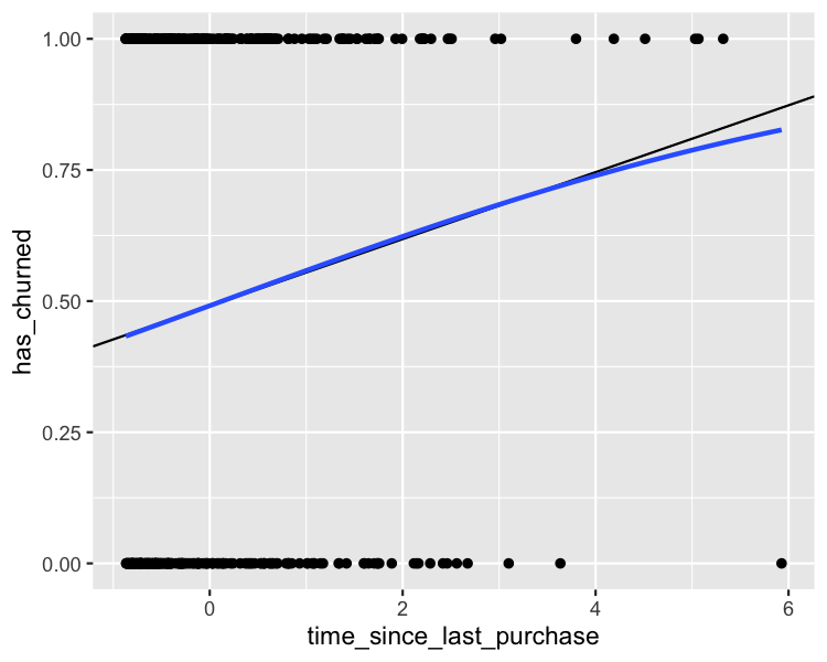
顧客が解約したか否かと最終購入からの経過時間の散布図。線形とロジスティックのトレンド線を表示。経過時間が長いほど解約確率が上がる。高い経過時間では2本の線に差が出る。

ズームアウト

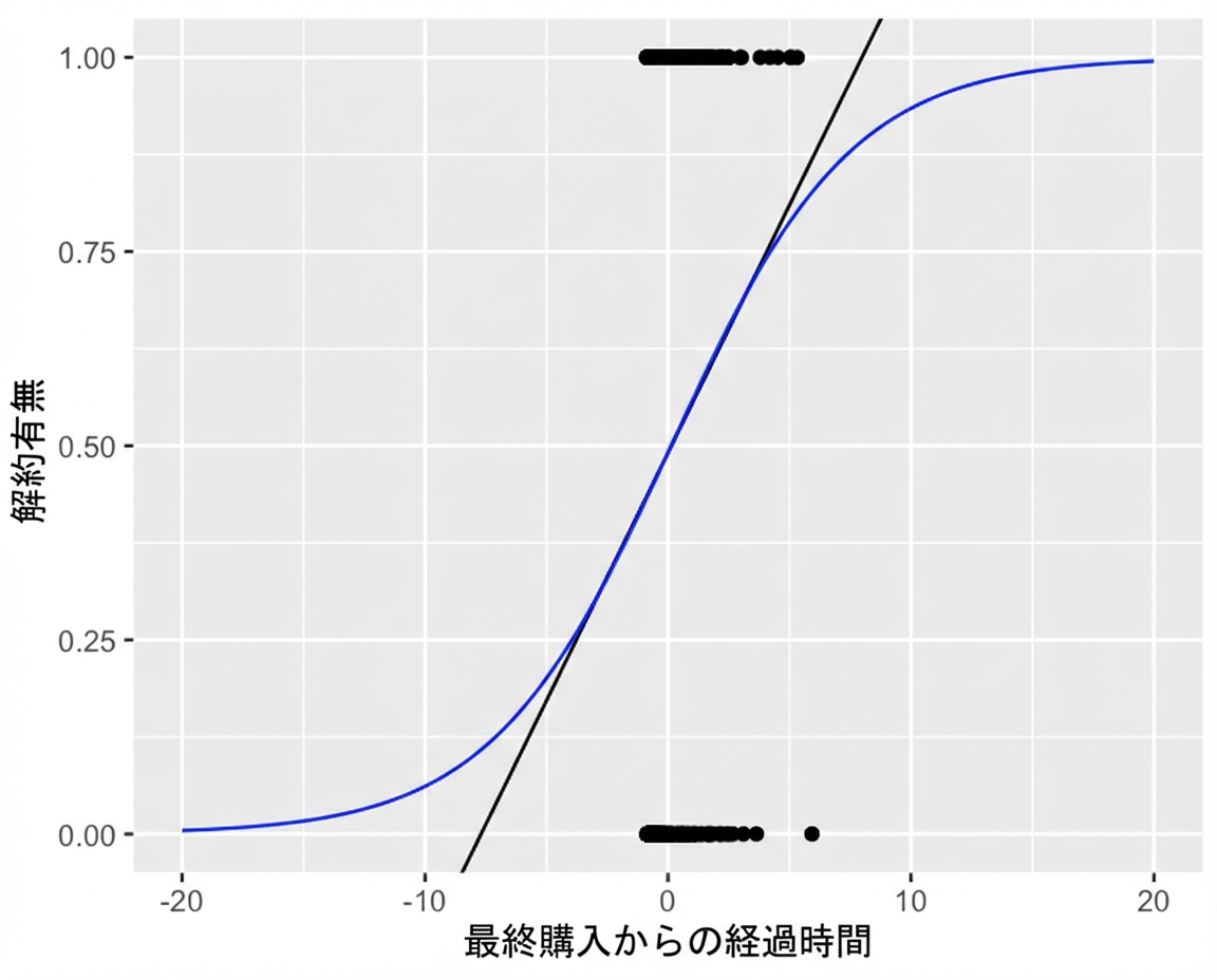
前図と同じ散布図（両トレンド線あり）。軸を広げて表示し、ロジスティックのトレンド線は解約確率の範囲0〜1を外れないことがわかる。

Passons à la pratique !

Rで学ぶ回帰入門