平均への回帰

Rで学ぶ回帰入門

Richie Cotton

Data Evangelist

概念

応答値 = 当てはめ値 + 残差
「説明できた部分」+「説明できなかった部分」
残差はモデルの問題と本質的なランダム性の双方で生じる
極端な事例は多くが偶然による
平均への回帰とは、極端な事例が時間とともに平均に近づくこと

ピアソンの父子データセット

父子ペア 1078 組
背の高い父には背の高い息子が多いか？

father_height_cm	son_height_cm
165.2	151.8
160.7	160.6
165.0	160.9
167.0	159.5
155.3	163.3
...	...

¹ Adapted from https://www.rdocumentation.org/packages/UsingR/topics/father.son

散布図

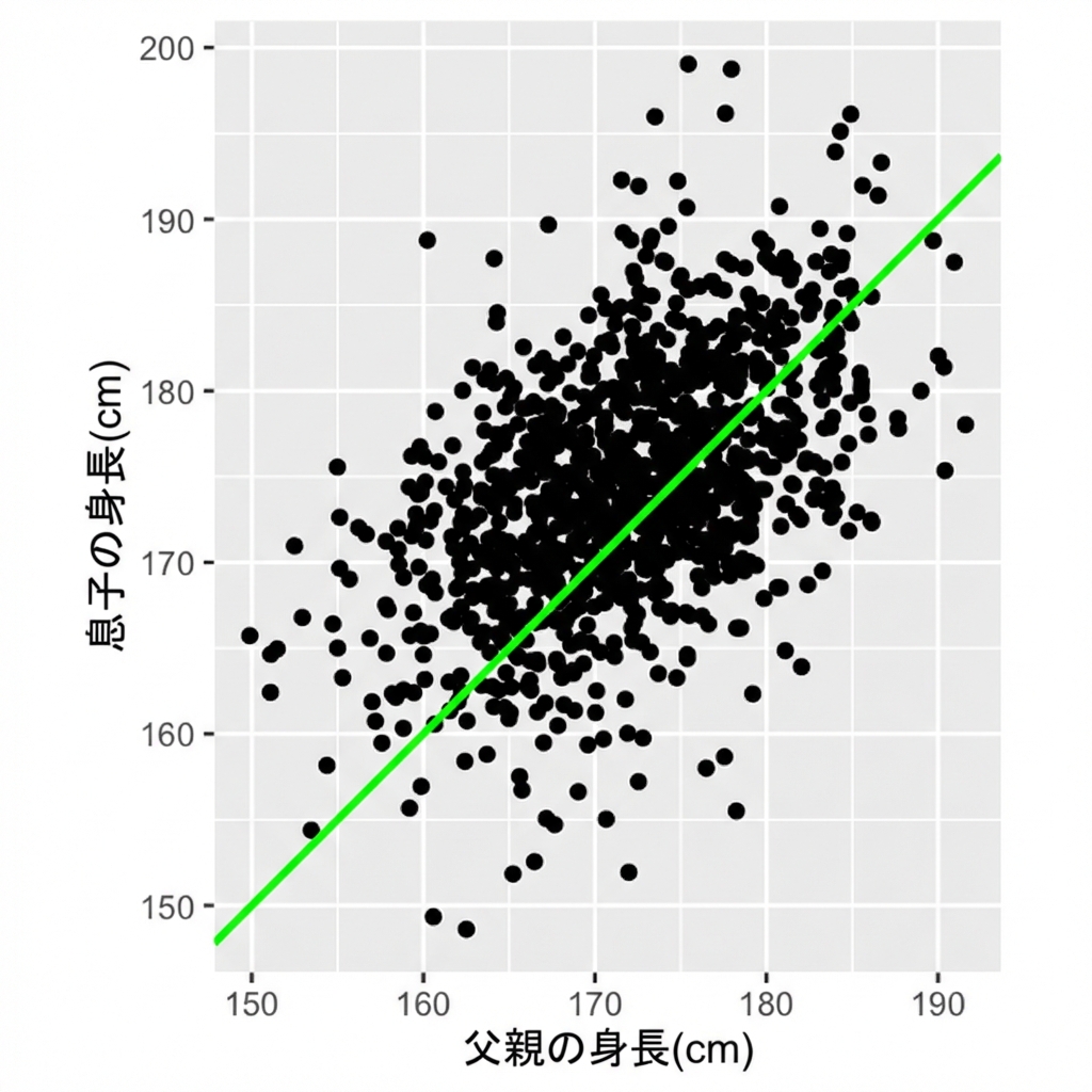
plt_son_vs_father <- ggplot(
  father_son, 
  aes(father_height_cm, son_height_cm)
) +
  geom_point() +
  geom_abline(color = "green", size = 1) +
  coord_fixed()

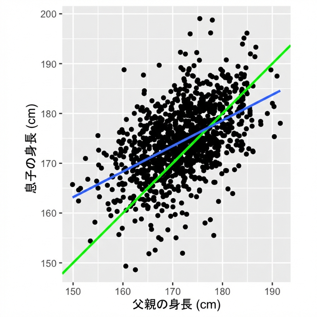
父の身長に対する息子の身長の散布図。父子が同じ身長となる線付き。父の身長が高いほど、息子も高い。

回帰直線の追加

plt_son_vs_father +
  geom_smooth(method = "lm", se = FALSE)

父の身長に対する息子の身長の散布図。線形トレンド線付き。トレンド線は、父子が同じ身長になる線より傾きが緩い。

回帰の実行

mdl_son_vs_father <- lm(
  son_height_cm ~ father_height_cm, 
  data = father_son
)

Call:
lm(formula = son_height_cm ~ father_height_cm, data = father_son)

Coefficients:
     (Intercept)  father_height_cm  
          86.072             0.514

予測の作成

really_tall_father <- tibble(
  father_height_cm = 190
)
predict(mdl_son_vs_father, really_tall_father)

183.7

really_short_father <- tibble(
  father_height_cm = 150
)
predict(mdl_son_vs_father, really_short_father)

163.2

Passons à la pratique !

Rで学ぶ回帰入門