外れ値、レバレッジ、影響度

Pythonで学ぶstatsmodelsによる回帰入門

Maarten Van den Broeck

Content Developer at DataCamp

ローチのデータセット

roach = fish[fish['species'] == "Roach"]
print(roach.head())

   species  mass_g  length_cm
35   Roach    40.0       12.9
36   Roach    69.0       16.5
37   Roach    78.0       17.5
38   Roach    87.0       18.2
39   Roach   120.0       18.6

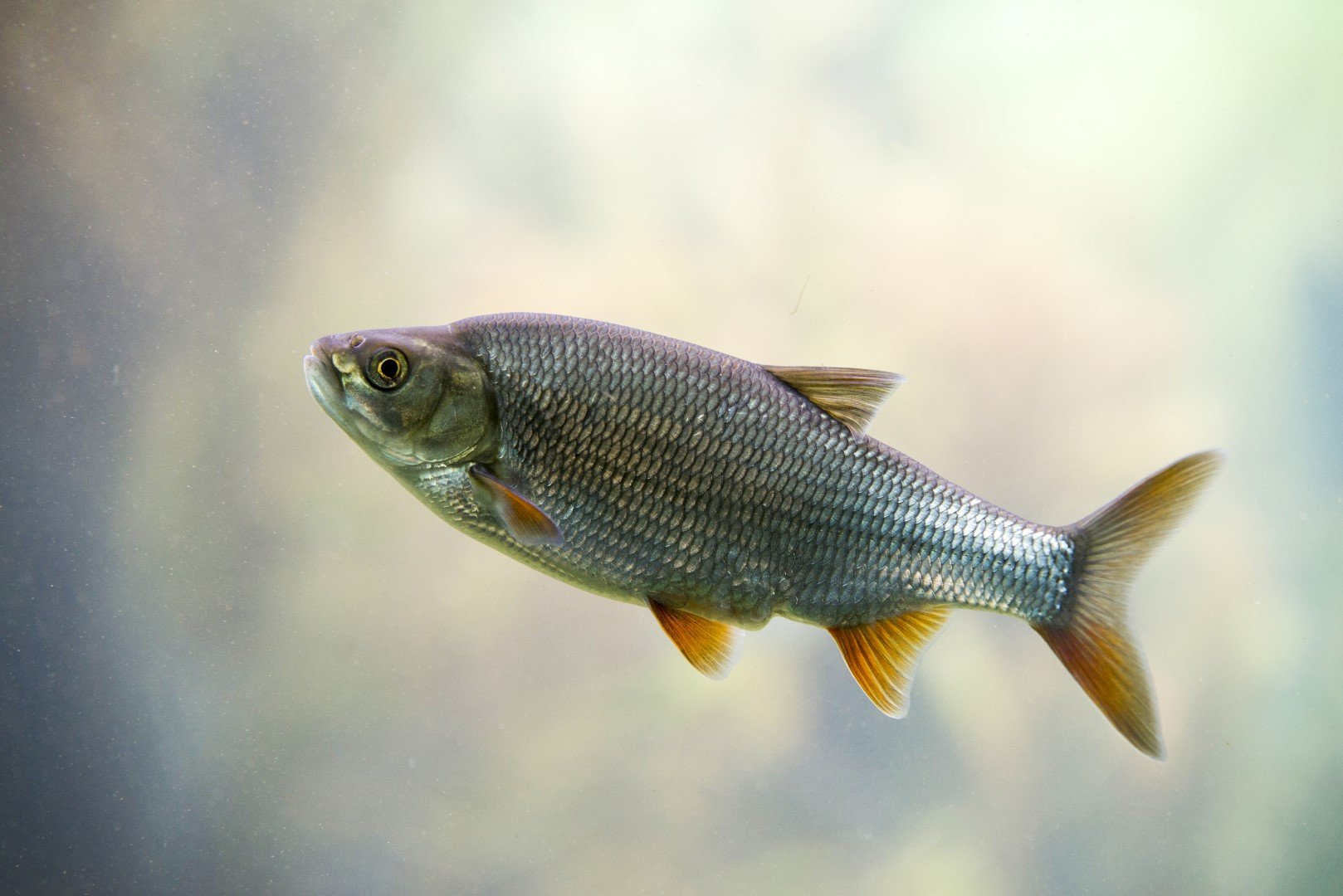
コイ科のローチ

どの点が外れ値か？

sns.regplot(x="length_cm",
            y="mass_g",
            data=roach,
            ci=None)
plt.show()

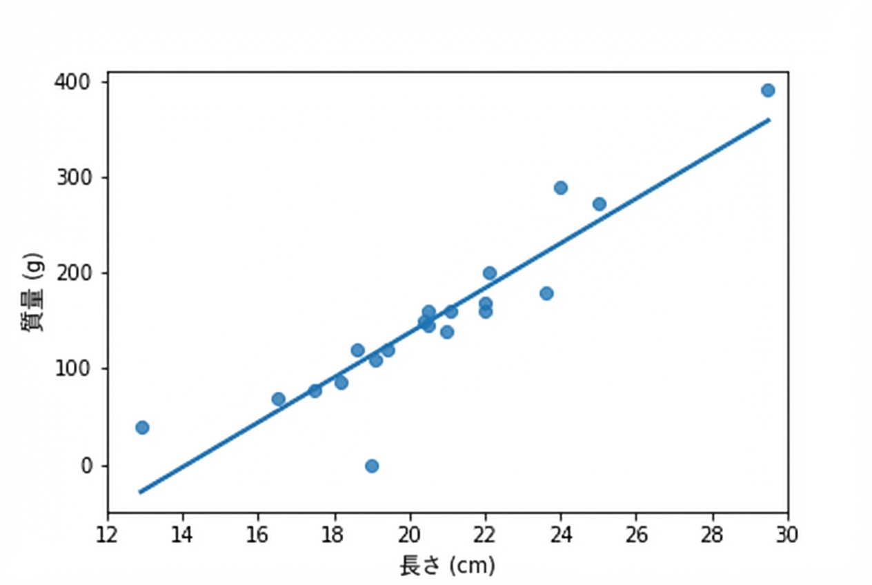
トレンド線付きの、ローチの長さに対する質量の散布図。多くの点はトレンド線に近い。

極端な説明変数の値

roach["extreme_l"] = ((roach["length_cm"] < 15) |
                    (roach["length_cm"] > 26))

fig = plt.figure()
sns.regplot(x="length_cm",
            y="mass_g",
            data=roach,
            ci=None)

sns.scatterplot(x="length_cm",
                y="mass_g",
                hue="extreme_l",
                data=roach)

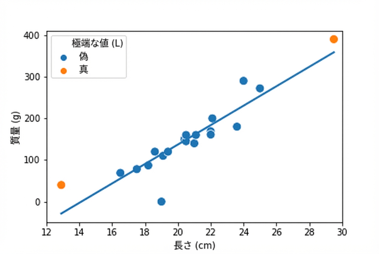
トレンド線付きの、ローチの長さに対する質量の散布図。多くは青だが、非常に短い個体と非常に長い個体はオレンジ。

回帰直線から離れた応答値

roach["extreme_m"] = roach["mass_g"] < 1

fig = plt.figure()
sns.regplot(x="length_cm",
            y="mass_g",
            data=roach,
            ci=None)

sns.scatterplot(x="length_cm",
                y="mass_g",
                hue="extreme_l",
                style="extreme_m",
                data=roach)

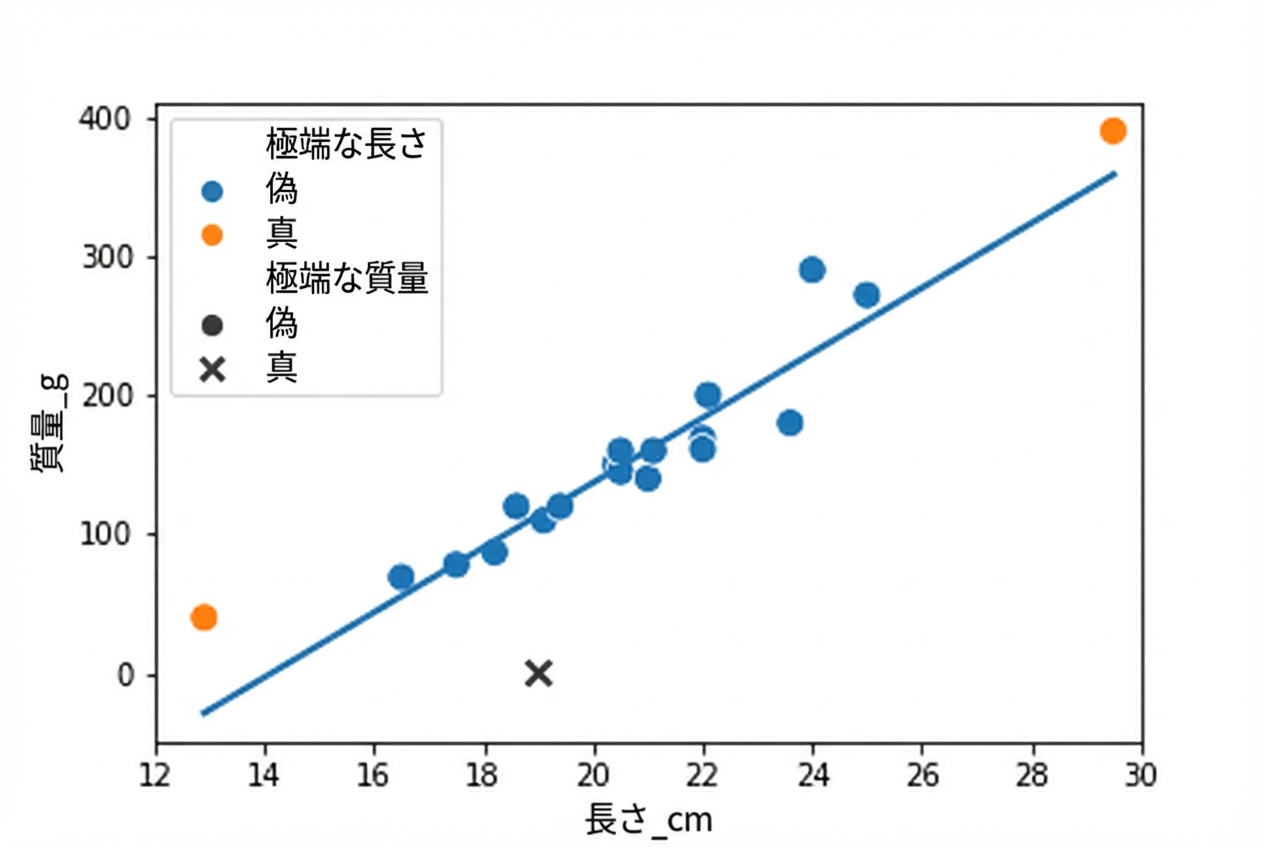
トレンド線付きの、ローチの長さに対する質量の散布図。多くは青だが、非常に短い個体と非常に長い個体はオレンジ。多くは丸印だが、見かけ上質量0の魚はバツ印。

レバレッジと影響度

「レバレッジ」は、説明変数の値がどれだけ極端かの尺度です。

「影響度」は、モデリング時にその観測を除外した場合にモデルがどれだけ変わるかを測ります。

レンチを回す人

.get_influence() と .summary_frame()

mdl_roach = ols("mass_g ~ length_cm", data=roach).fit()

summary_roach = mdl_roach.get_influence().summary_frame()

roach["leverage"] = summary_roach["hat_diag"]

print(roach.head())

   species  mass_g  length_cm  leverage
35   Roach    40.0       12.9  0.313729
36   Roach    69.0       16.5  0.125538
37   Roach    78.0       17.5  0.093487
38   Roach    87.0       18.2  0.076283
39   Roach   120.0       18.6  0.068387

クックの距離

最も一般的な影響度の尺度は「クックの距離」です。

roach["cooks_dist"] = summary_roach["cooks_d"]
print(roach.head())

   species  mass_g  length_cm  leverage  cooks_dist
35   Roach    40.0       12.9  0.313729    1.074015
36   Roach    69.0       16.5  0.125538    0.010429
37   Roach    78.0       17.5  0.093487    0.000020
38   Roach    87.0       18.2  0.076283    0.001980
39   Roach   120.0       18.6  0.068387    0.006610

影響度が高いローチ

print(roach.sort_values("cooks_dist", ascending = False))

   species  mass_g  length_cm  leverage  cooks_dist
35   Roach    40.0       12.9  0.313729    1.074015 # 非常に短いローチ
54   Roach   390.0       29.5  0.394740    0.365782 # 非常に長いローチ
40   Roach     0.0       19.0  0.061897    0.311852 # 質量0のローチ
52   Roach   290.0       24.0  0.099488    0.150064
51   Roach   180.0       23.6  0.088391    0.061209
..     ...     ...        ...       ...         ...
43   Roach   150.0       20.4  0.050264    0.000257
44   Roach   145.0       20.5  0.050092    0.000256
42   Roach   120.0       19.4  0.056815    0.000199
47   Roach   160.0       21.1  0.050910    0.000137
37   Roach    78.0       17.5  0.093487    0.000020

最も影響度の高い個体を除外

roach_not_short = roach[roach["length_cm"] != 12.9]

sns.regplot(x="length_cm",
            y="mass_g",
            data=roach,
            ci=None,
            line_kws={"color": "green"})

sns.regplot(x="length_cm",
            y="mass_g",
            data=roach_not_short,
            ci=None,
            line_kws={"color": "red"})

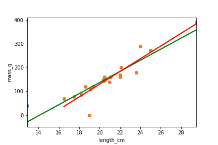
ローチの長さに対する質量の散布図と2本のトレンド線。1本は全データ、もう1本は最短個体を除外。後者は明らかに勾配が急。

Passons à la pratique !

Pythonで学ぶstatsmodelsによる回帰入門