時系列間の関係：相関

Pythonでの時系列データ操作

Stefan Jansen

Founder & Lead Data Scientist at Applied Artificial Intelligence

相関と系列間の関係

これまでは各変数の特徴に注目
ここからは変数間の関係の特徴
相関：線形関係を測定
金融市場：予測とリスク管理で重要
pandas と seaborn で計算・可視化可能

相関と線形関係

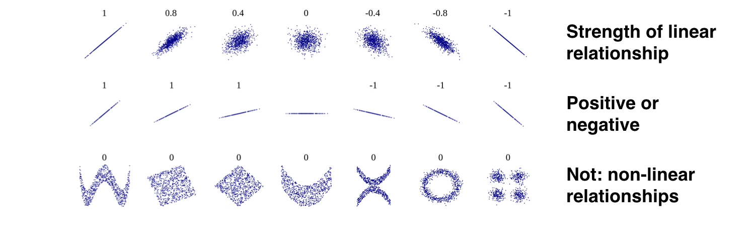
相関係数：2変数が平均の周りでどれだけ同調して動くか
範囲は -1 〜 +1 $\ \ \ \ \ r = \frac{\sum_{i=1}^{N} (x_i - \bar{x})(y_i - \bar{y})}{s_xs_y}$

ch3_4_v2 - Correlation & Heatmaps.011.png

5つの価格時系列をインポート

data = pd.read_csv('assets.csv', parse_dates=['date'], 
                   index_col='date')

data = data.dropna().info()

DatetimeIndex: 2469 entries, 2007-05-25 to 2017-05-22
Data columns (total 5 columns):
sp500     2469 non-null float64
nasdaq    2469 non-null float64
bonds     2469 non-null float64
gold      2469 non-null float64
oil       2469 non-null float64

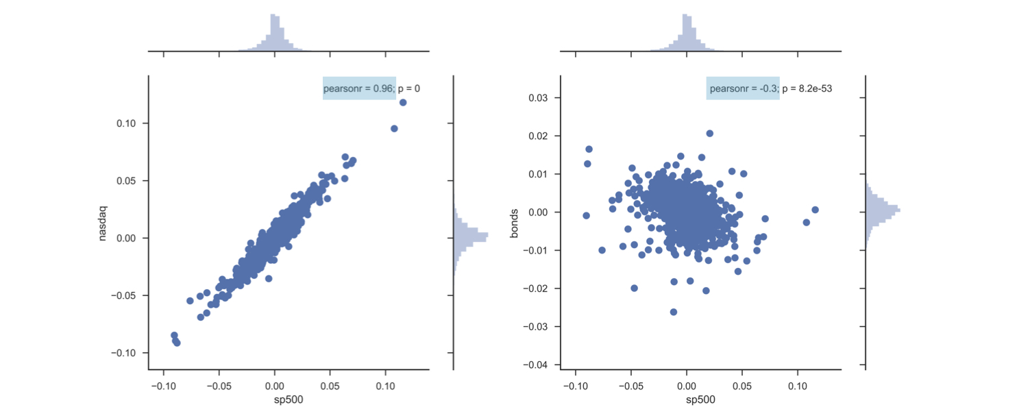
ペアの線形関係を可視化

daily_returns = data.pct_change()

sns.jointplot(x='sp500', y='nasdaq', data=data_returns);

ch3_4_v2 - Correlation & Heatmaps.015.png

相関を一括計算

correlations = returns.corr()

correlations

bonds       oil      gold     sp500    nasdaq
bonds   1.000000 -0.183755  0.003167 -0.300877 -0.306437
oil    -0.183755  1.000000  0.105930  0.335578  0.289590
gold    0.003167  0.105930  1.000000 -0.007786 -0.002544
sp500  -0.300877  0.335578 -0.007786  1.000000  0.959990
nasdaq -0.306437  0.289590 -0.002544  0.959990  1.000000

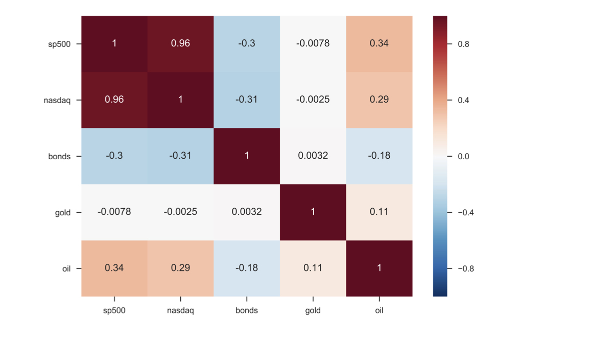
相関を一望で可視化

sns.heatmap(correlations, annot=True)

ch3_4_v2 - Correlation & Heatmaps.019.png

Passons à la pratique !

Pythonでの時系列データ操作