インデックスの相関とExcelへのエクスポート

Pythonでの時系列データ操作

Stefan Jansen

Founder & Lead Data Scientist at Applied Artificial Intelligence

インデックスの追加分析

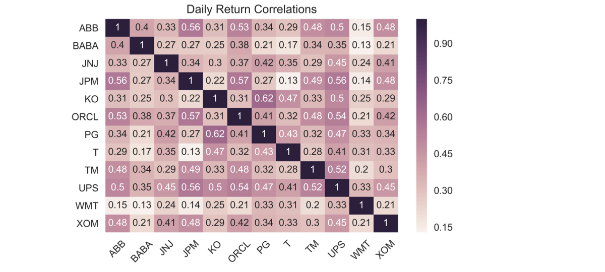
日次リターンの相関:
すべての構成要素で計算
ヒートマップで可視化
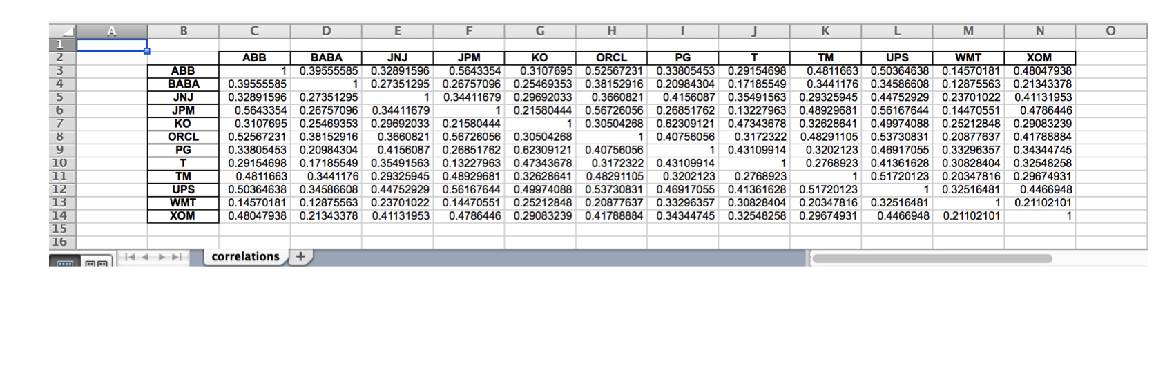
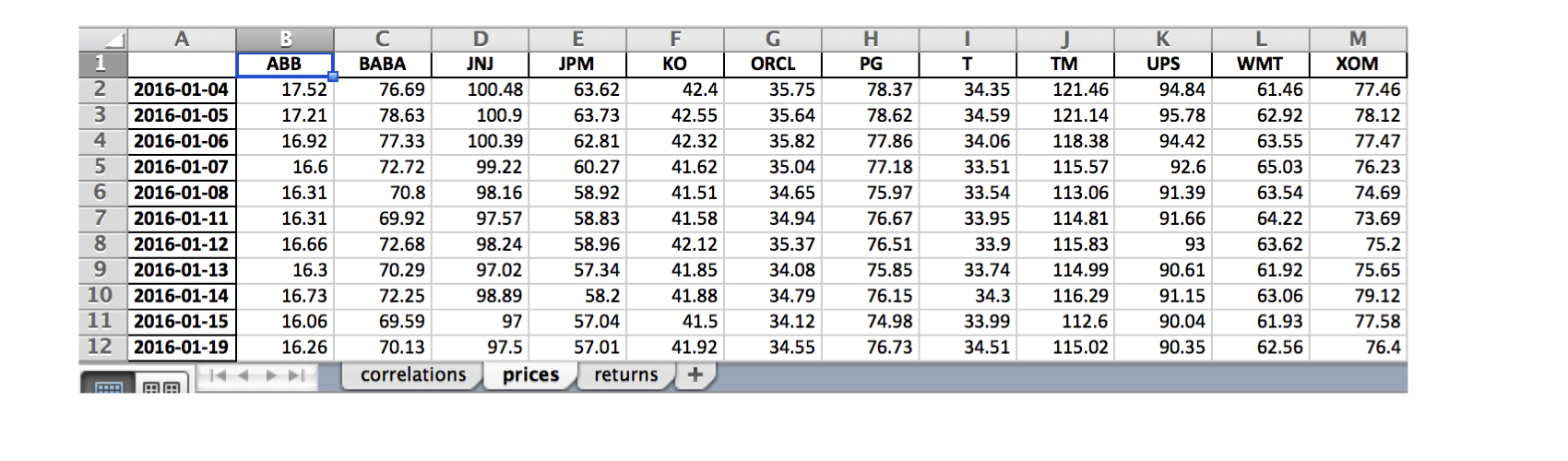
結果を.xlsと.xlsxで出力:
単一ワークシート
複数ワークシート

インデックス構成銘柄 - 価格データ

data = DataReader(tickers, 'google', start='2016', end='2017')['Close']

data.info()

DatetimeIndex: 252 entries, 2016-01-04 to 2016-12-30
Data columns (total 12 columns):
ABB     252 non-null float64
BABA    252 non-null float64
JNJ     252 non-null float64
JPM     252 non-null float64
KO      252 non-null float64
ORCL    252 non-null float64
PG      252 non-null float64
T       252 non-null float64
TM      252 non-null float64
UPS     252 non-null float64
WMT     252 non-null float64
XOM     252 non-null float64

インデックス構成銘柄: リターン相関

daily_returns = data.pct_change()

correlations = daily_returns.corr()

ABB  BABA  JNJ  JPM   KO  ORCL   PG    T   TM  UPS  WMT  XOM
ABB  1.00  0.40 0.33 0.56 0.31  0.53 0.34 0.29 0.48 0.50 0.15 0.48
BABA 0.40  1.00 0.27 0.27 0.25  0.38 0.21 0.17 0.34 0.35 0.13 0.21
JNJ  0.33  0.27 1.00 0.34 0.30  0.37 0.42 0.35 0.29 0.45 0.24 0.41
JPM  0.56  0.27 0.34 1.00 0.22  0.57 0.27 0.13 0.49 0.56 0.14 0.48
KO   0.31  0.25 0.30 0.22 1.00  0.31 0.62 0.47 0.33 0.50 0.25 0.29
ORCL 0.53  0.38 0.37 0.57 0.31  1.00 0.41 0.32 0.48 0.54 0.21 0.42
PG   0.34  0.21 0.42 0.27 0.62  0.41 1.00 0.43 0.32 0.47 0.33 0.34
T    0.29  0.17 0.35 0.13 0.47  0.32 0.43 1.00 0.28 0.41 0.31 0.33
TM   0.48  0.34 0.29 0.49 0.33  0.48 0.32 0.28 1.00 0.52 0.20 0.30
UPS  0.50  0.35 0.45 0.56 0.50  0.54 0.47 0.41 0.52 1.00 0.33 0.45
WMT  0.15  0.13 0.24 0.14 0.25  0.21 0.33 0.31 0.20 0.33 1.00 0.21
XOM  0.48  0.21 0.41 0.48 0.29  0.42 0.34 0.33 0.30 0.45 0.21 1.00

インデックス構成銘柄: リターン相関

sns.heatmap(correlations, annot=True)
plt.xticks(rotation=45)
plt.title('Daily Return Correlations')

ch4_4_v2 - Index Correlation & Saving Results to Excel.010.png

単一のExcelワークシートに保存

correlations.to_excel(excel_writer= 'correlations.xls',
                      sheet_name='correlations',
                      startrow=1,
                      startcol=1)

ch4_4_v2 - Index Correlation & Saving Results to Excel.012.png

複数のExcelワークシートに保存

data.index = data.index.date # Keep only date component

with pd.ExcelWriter('stock_data.xlsx') as writer:

    corr.to_excel(excel_writer=writer, sheet_name='correlations')

    data.to_excel(excel_writer=writer, sheet_name='prices')

    data.pct_change().to_excel(writer, sheet_name='returns')

ch4_4_v2 - Index Correlation & Saving Results to Excel.015.png

演習に進みましょう

Pythonでの時系列データ操作