時系列の成長率を比較する

Pythonでの時系列データ操作

Stefan Jansen

Founder & Lead Data Scientist at Applied Artificial Intelligence

株式のパフォーマンスを比較する

株価系列: 水準が違うと比較が難しい
解決策: 価格系列を開始値100に正規化
全価格を系列の初値で割り、100を掛ける
- 同じ開始点
- すべて開始点に対する相対値
- 開始点からの差をパーセントポイントで表現

単一系列の正規化 (1)

google = pd.read_csv('google.csv', parse_dates=['date'], index_col='date')

google.head(3)

             price
date
2010-01-04  313.06
2010-01-05  311.68
2010-01-06  303.83

first_price = google.price.iloc[0]  # int-based selection

first_price

313.06

first_price == google.loc('2010-01-04', 'price')

True

単一系列の正規化 (2)

normalized = google.price.div(first_price).mul(100)

normalized.plot(title='Google Normalized Series')

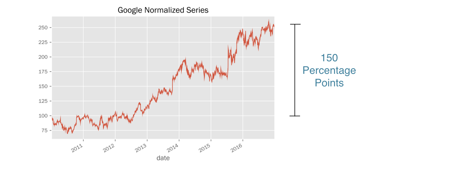
ch2_1_v2 - Compare Time Series Trends.017.png

複数系列の正規化 (1)

prices = pd.read_csv('stock_prices.csv',
                     parse_dates=['date'],
                     index_col='date')

prices.info()

DatetimeIndex: 1761 entries, 2010-01-04 to 2016-12-30
Data columns (total 3 columns):
AAPL    1761 non-null float64
GOOG    1761 non-null float64
YHOO    1761 non-null float64
dtypes: float64(3)

prices.head(2)

             AAPL    GOOG   YHOO
Date
2010-01-04  30.57  313.06  17.10
2010-01-05  30.63  311.68  17.23

複数系列の正規化 (2)

prices.iloc[0]

AAPL     30.57
GOOG    313.06
YHOO     17.10
Name: 2010-01-04 00:00:00, dtype: float64

normalized = prices.div(prices.iloc[0])

normalized.head(3)

                AAPL      GOOG      YHOO
Date
2010-01-04  1.000000  1.000000  1.000000
2010-01-05  1.001963  0.995592  1.007602
2010-01-06  0.985934  0.970517  1.004094

.div(): SeriesのインデックスとDataFrame列を自動的に整列

ベンチマークとの比較 (1)

index = pd.read_csv('benchmark.csv', parse_dates=['date'], index_col='date')

index.info()

DatetimeIndex: 1826 entries, 2010-01-01 to 2016-12-30
Data columns (total 1 columns):
SP500    1762 non-null float64
dtypes: float64(1)

prices = pd.concat([prices, index], axis=1).dropna()

prices.info()

DatetimeIndex: 1761 entries, 2010-01-04 to 2016-12-30
Data columns (total 4 columns):
AAPL     1761 non-null float64
GOOG     1761 non-null float64
YHOO     1761 non-null float64
SP500    1761 non-null float64
dtypes: float64(4)

ベンチマークとの比較 (2)

prices.head(1)

             AAPL    GOOG   YHOO    SP500
2010-01-04  30.57  313.06  17.10  1132.99

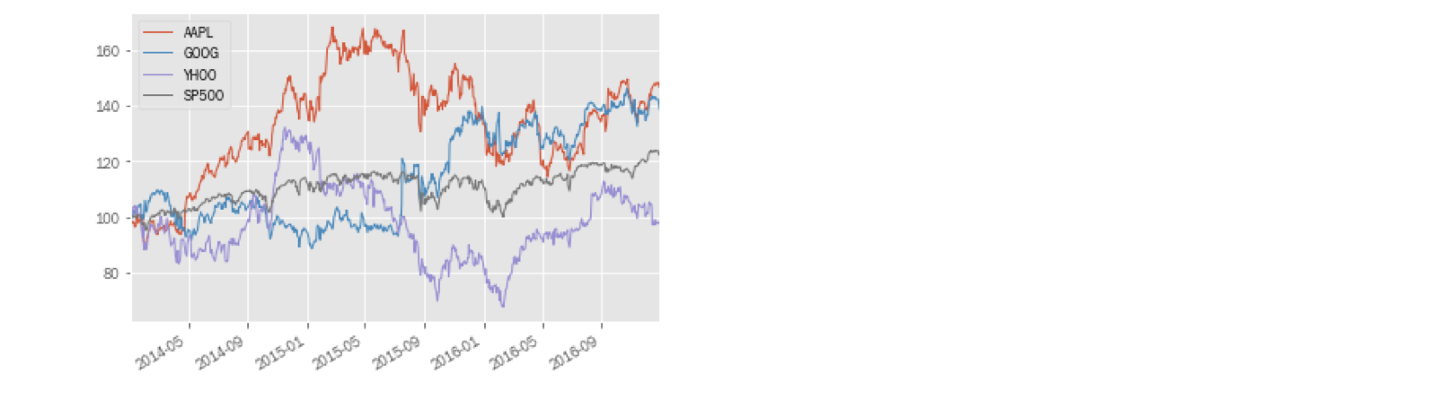
normalized = prices.div(prices.iloc[0]).mul(100)

normalized.plot()

ch2_1_v2 - Compare Time Series Trends.031.png

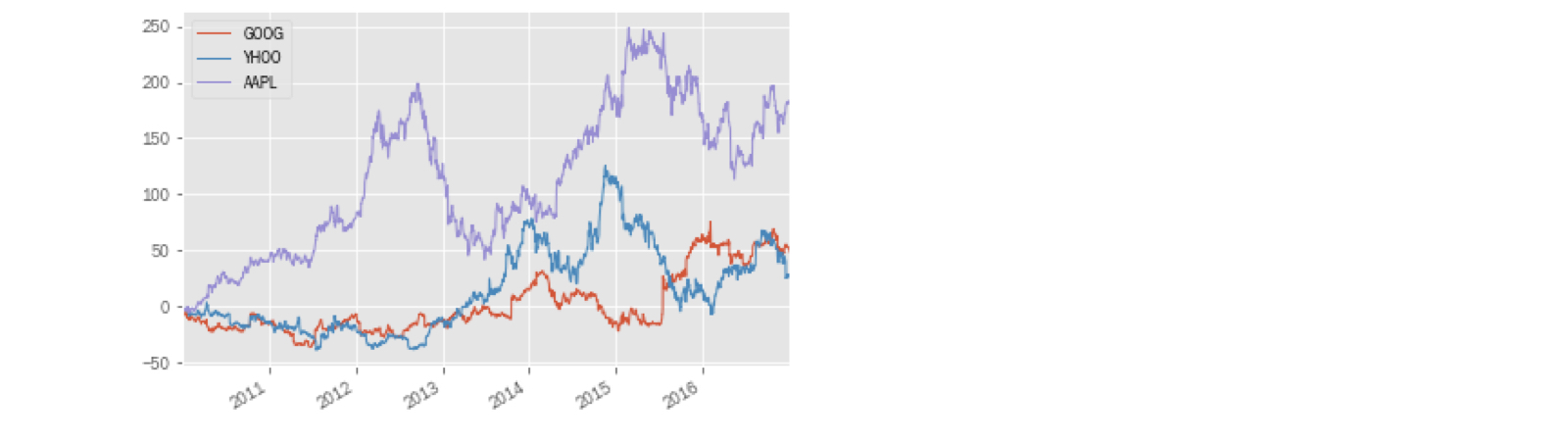
パフォーマンス差のプロット

diff = normalized[tickers].sub(normalized['SP500'], axis=0)

                GOOG      YHOO      AAPL
2010-01-04  0.000000  0.000000  0.000000
2010-01-05 -0.752375  0.448669 -0.115294
2010-01-06 -3.314604  0.043069 -1.772895

.sub(..., axis=0): インデックスを揃えて、各列から Series を減算

パフォーマンス差のプロット

diff.plot()

ch2_1_v2 - Compare Time Series Trends.035.png

Passons à la pratique !

Pythonでの時系列データ操作