이상치, 레버리지, 영향력

R로 시작하는 회귀 분석

Richie Cotton

Data Evangelist at DataCamp

Roach 데이터셋

roach <- fish %>%
  filter(species == "Roach")

species	length_cm	mass_g
Roach	12.9	40
Roach	16.5	69
Roach	17.5	78
Roach	18.2	87
Roach	18.6	120
...	...	...

어떤 점이 이상치인가요?

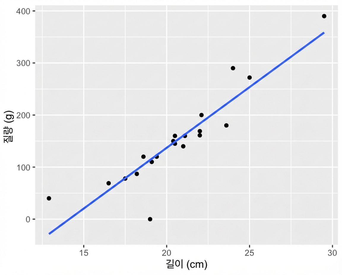
ggplot(roach, aes(length_cm, mass_g)) +
  geom_point() +
  geom_smooth(method = "lm", se = FALSE)

바퀴벌레 길이 대비 질량 산점도와 추세선. 대부분의 점이 추세선을 밀접히 따른다.

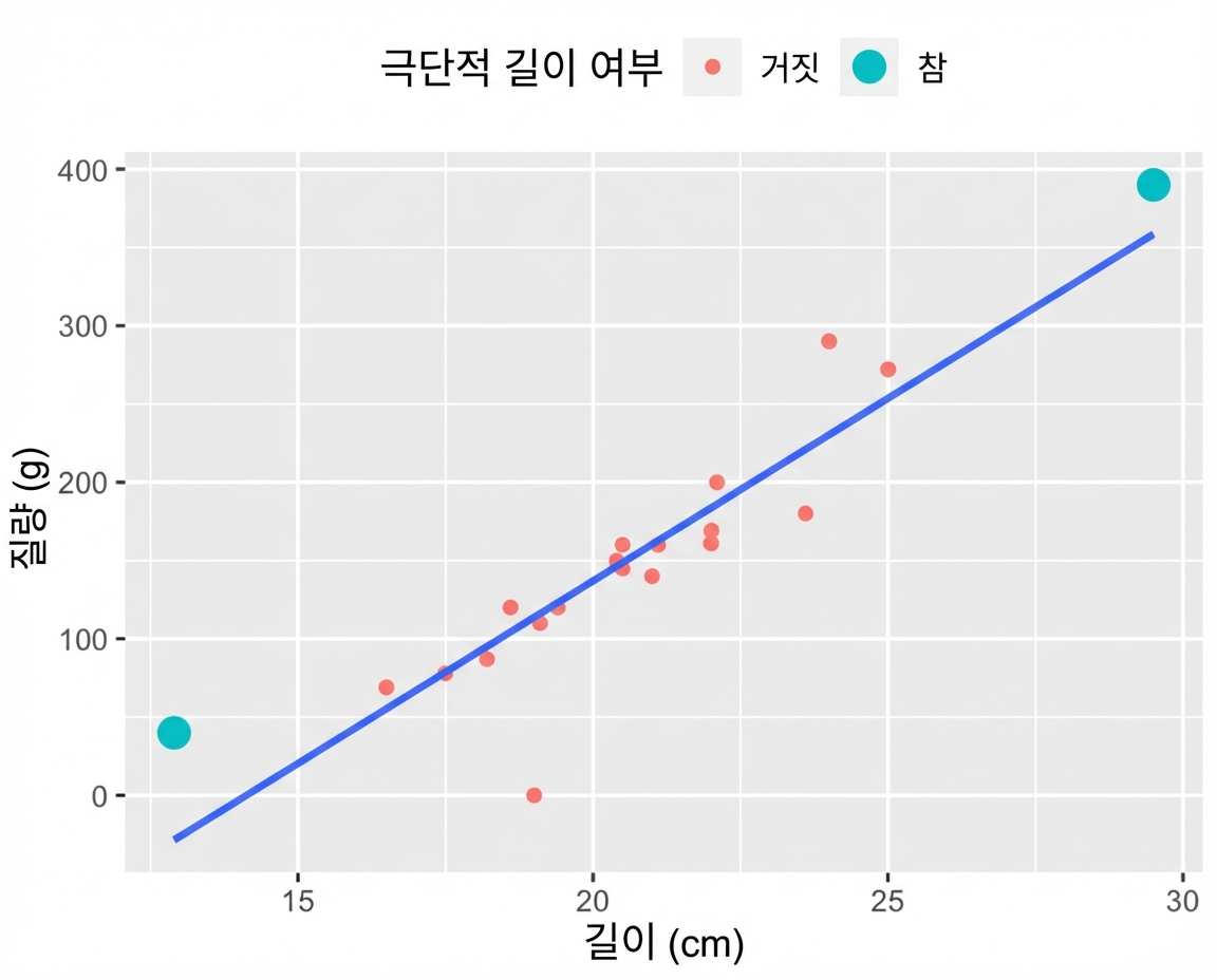
극단적 설명변수 값

roach %>% 
  mutate(
    has_extreme_length = length_cm < 15 | length_cm > 26
  ) %>% 
  ggplot(aes(length_cm, mass_g)) +
  geom_point(aes(color = has_extreme_length)) +
  geom_smooth(method = "lm", se = FALSE)

바퀴벌레 길이 대비 질량 산점도와 추세선. 대부분의 점은 빨간색이지만, 매우 짧은 개체와 매우 긴 개체 두 점은 청록색이다.

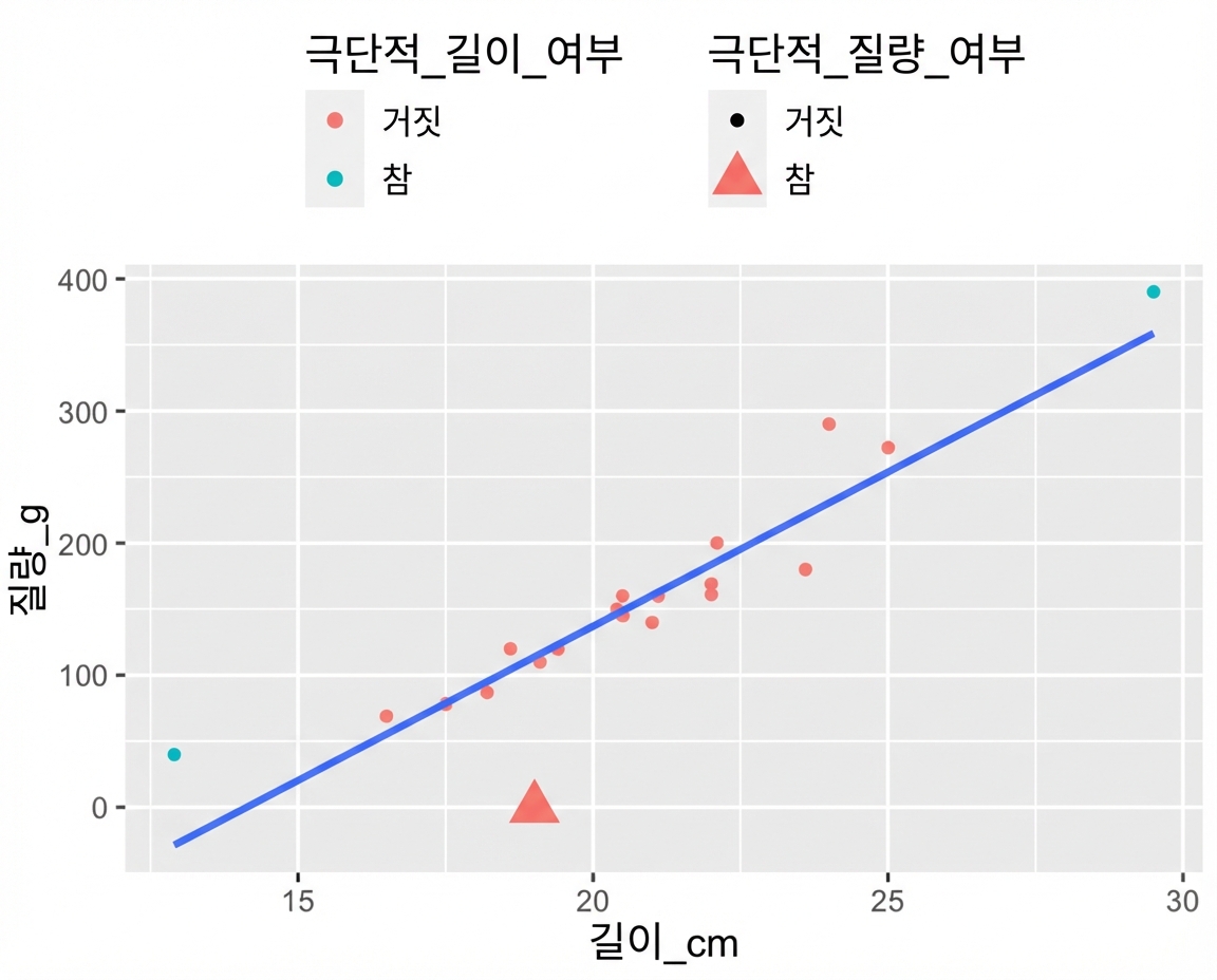
회귀선에서 멀리 떨어진 반응값

roach %>% 
  mutate(
    has_extreme_length = length_cm < 15 | length_cm > 26,
    has_extreme_mass = mass_g < 1
  ) %>% 
  ggplot(aes(length_cm, mass_g)) +
  geom_point(
    aes(
      color = has_extreme_length, 
      shape = has_extreme_mass
    )
  ) +
  geom_smooth(method = "lm", se = FALSE)

바퀴벌레 길이 대비 질량 산점도와 추세선. 대부분의 점은 빨간색이며, 매우 짧은 개체와 매우 긴 개체 두 점은 청록색이다. 대부분 원형이지만, 질량이 0으로 보이는 개체 하나는 삼각형이다.

레버리지

레버리지는 설명변수 값이 얼마나 극단적인지의 척도입니다.

mdl_roach <- lm(mass_g ~ length_cm, data = roach)

hatvalues(mdl_roach)

     1      2      3      4      5      6      7 
0.3137 0.1255 0.0935 0.0763 0.0684 0.0619 0.0605 
     8      9     10     11     12     13     14 
0.0568 0.0503 0.0501 0.0501 0.0506 0.0509 0.0581 
    15     16     17     18     19     20 
0.0581 0.0593 0.0884 0.0995 0.1334 0.3947

.hat 열

library(broom)
augment(mdl_roach)

# A tibble: 20 × 8
   mass_g length_cm .fitted   .resid   .hat .sigma   .cooksd .std.resid
    <dbl>     <dbl>   <dbl>    <dbl>  <dbl>  <dbl>     <dbl>      <dbl>
 1     40      12.9   -28.6   68.6   0.314    33.8 1.07          2.17  
 2     69      16.5    55.4   13.6   0.126    39.1 0.0104        0.381 
 3     78      17.5    78.7   -0.711 0.0935   39.3 0.0000197    -0.0196
 4     87      18.2    95.0   -8.03  0.0763   39.2 0.00198      -0.219 
 5    120      18.6   104.    15.6   0.0684   39.1 0.00661       0.424 
...

레버리지가 큰 개체

mdl_roach %>%
  augment() %>%
  select(mass_g, length_cm, leverage = .hat) %>%
  arrange(desc(leverage)) %>% 
  head()

# A tibble: 6 x 3
  mass_g length_cm leverage
   <dbl>     <dbl>    <dbl>
1    390      29.5   0.395  # 매우 긴 개체
2     40      12.9   0.314  # 매우 짧은 개체
3    272      25     0.133 
4     69      16.5   0.126 
5    290      24     0.0995
6     78      17.5   0.0935

영향력

영향력은 해당 관측치를 제외하고 모델링했을 때 모델이 얼마나 달라지는지를 측정합니다.

렌치를 돌리는 사람

Cook의 거리

Cook의 거리(Cook's distance)는 가장 일반적인 영향력 지표입니다.

cooks.distance(mdl_roach)

       1        2        3        4        5        6 
1.07e+00 1.04e-02 1.97e-05 1.98e-03 6.61e-03 3.12e-01 
       7        8        9       10       11       12 
8.53e-04 1.99e-04 2.57e-04 2.56e-04 2.45e-03 7.95e-03 
      13       14       15       16       17       18 
1.37e-04 4.82e-03 1.15e-02 4.52e-03 6.12e-02 1.50e-01 
      19       20 
2.06e-02 3.66e-01

.cooksd 열

library(broom)
augment(mdl_roach)

# A tibble: 20 x 9
   mass_g length_cm .fitted .se.fit   .resid   .hat .sigma   .cooksd .std.resid
    <dbl>     <dbl>   <dbl>   <dbl>    <dbl>  <dbl>  <dbl>     <dbl>      <dbl>
 1     40      12.9   -28.6   21.4    68.6   0.314    33.8 1.07          2.17  
 2     69      16.5    55.4   13.5    13.6   0.126    39.1 0.0104        0.381 
 3     78      17.5    78.7   11.7    -0.711 0.0935   39.3 0.0000197    -0.0196
 4     87      18.2    95.0   10.5    -8.03  0.0763   39.2 0.00198      -0.219 
 5    120      18.6   104.     9.98   15.6   0.0684   39.1 0.00661       0.424 
...

영향력이 큰 개체

mdl_roach %>%
  augment() %>%
  select(mass_g, length_cm, cooks_dist = .cooksd) %>%
  arrange(desc(cooks_dist)) %>% 
  head()

# A tibble: 6 x 3
  mass_g length_cm cooks_dist
   <dbl>     <dbl>      <dbl>
1     40      12.9     1.07   # 매우 짧은 개체
2    390      29.5     0.366  # 매우 긴 개체
3      0      19       0.312  # 질량 0 개체
4    290      24       0.150 
5    180      23.6     0.0612
6    272      25       0.0206

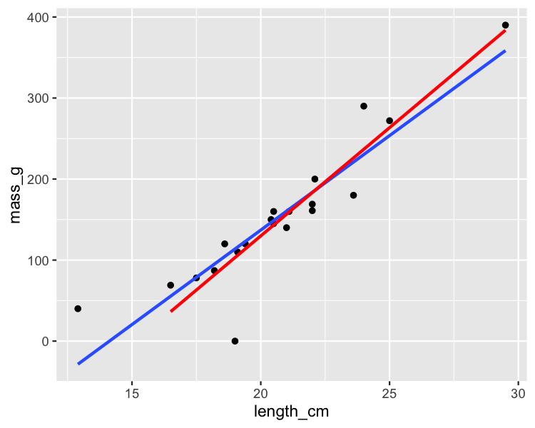
가장 영향력 큰 개체 제거하기

roach_not_short <- roach %>% 
  filter(length != 12.9)

ggplot(roach, aes(length_cm, mass_g)) +
  geom_point() +
  geom_smooth(method = "lm", se = FALSE) +
  geom_smooth(
    method = "lm", se = FALSE, 
    data = roach_not_short, color = "red"
  )

바퀴벌레 길이 대비 질량 산점도와 두 개의 추세선. 하나는 전체 데이터, 다른 하나는 가장 짧은 개체를 제외. 제외한 추세선이 더 가파르다.

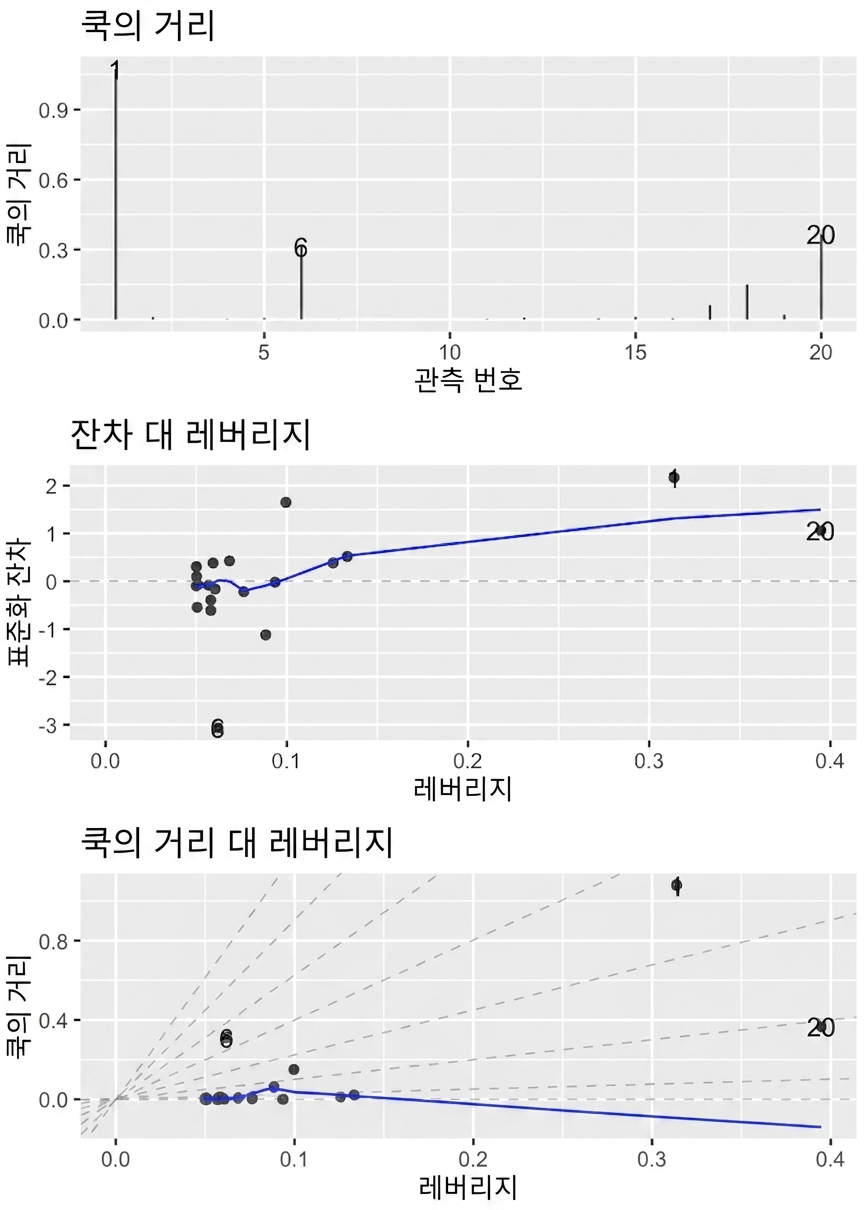
autoplot()

autoplot(
  mdl_roach, 
  which = 4:6, 
  nrow = 3,
  ncol = 1
)

세 개의 roach 모델 진단 플롯이 세 패널로 배치됨.

연습해 봅시다!

R로 시작하는 회귀 분석