예측하기

R로 시작하는 회귀 분석

Richie Cotton

Data Evangelist at DataCamp

fish 데이터셋: 도미

bream <- fish %>% 
  filter(species == "Bream")

species	length_cm	mass_g
Bream	23.2	242
Bream	24.0	290
Bream	23.9	340
Bream	26.3	363
Bream	26.5	430
...	...	...

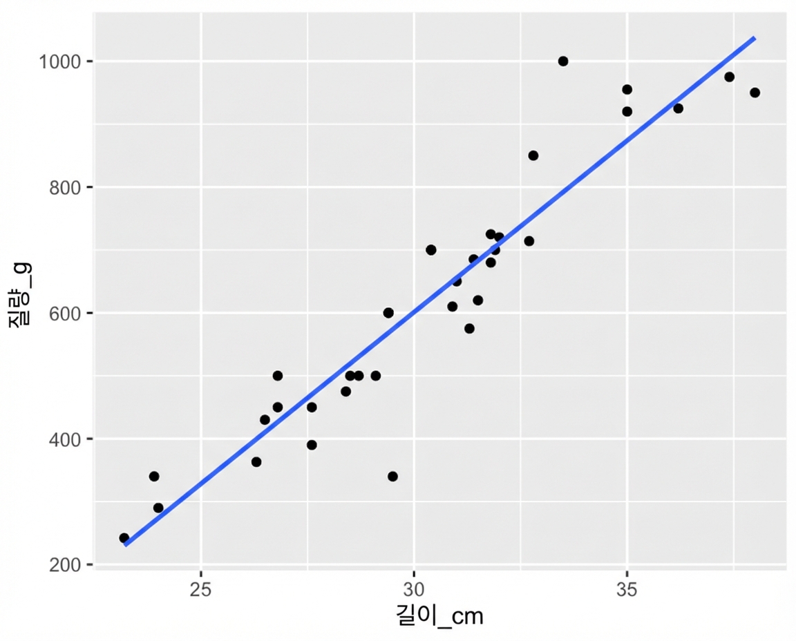
무게 vs. 길이 그리기

ggplot(bream, aes(length_cm, mass_g)) +
  geom_point() +
  geom_smooth(method = "lm", se = FALSE)

도미 길이 대비 무게 산점도와 선형 추세선. 점들은 모두 추세선에 가깝다.

모델 실행하기

mdl_mass_vs_length <- lm(mass_g ~ length_cm, data = bream)

Call:
lm(formula = mass_g ~ length_cm, data = bream)

Coefficients:
(Intercept)    length_cm  
   -1035.35        54.55

예측할 설명값 데이터

설명 변수를 이렇게 두면,
반응 변수는 어떤 값이 될까요?

library(dplyr)
explanatory_data <- tibble(length_cm = 20:40)

predict() 호출

library(tibble)
explanatory_data <- tibble(length_cm = 20:40)

predict(mdl_mass_vs_length, explanatory_data)

         1          2          3          4          5          6 
  55.65205  110.20203  164.75202  219.30200  273.85198  328.40196 
         7          8          9         10         11         12 
 382.95194  437.50192  492.05190  546.60188  601.15186  655.70184 
        13         14         15         16         17         18 
 710.25182  764.80181  819.35179  873.90177  928.45175  983.00173 
        19         20         21 
1037.55171 1092.10169 1146.65167

데이터 프레임에서 예측하기

library(dplyr)
explanatory_data <- tibble(length_cm = 20:40)

prediction_data <- explanatory_data %>% 
  mutate(
    mass_g = predict(
      mdl_mass_vs_length, explanatory_data
    )
  )

# A tibble: 21 x 2
   length_cm mass_g
       <int>  <dbl>
 1        20   55.7
 2        21  110. 
 3        22  165. 
 4        23  219. 
 5        24  274. 
 6        25  328. 
 7        26  383. 
 8        27  438. 
 9        28  492. 
10        29  547. 
# ... with 11 more rows

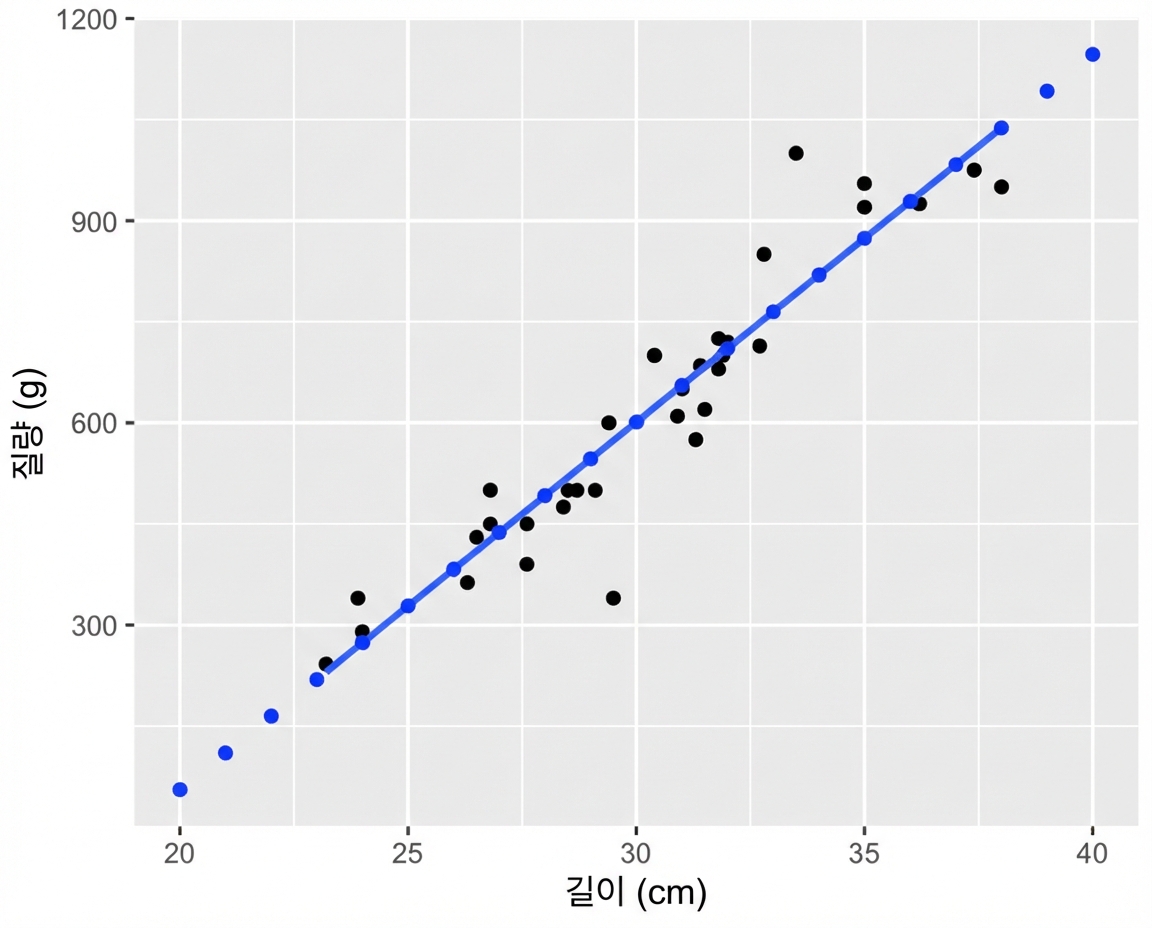
예측 표시하기

ggplot(bream, aes(length_cm, mass_g)) +
  geom_point() +
  geom_smooth(method = "lm", se = FALSE) +
  geom_point(
    data = prediction_data, 
    color = "blue"
  )

도미 길이 대비 무게 산점도와 선형 추세선. predict()로 계산한 점들이 주석으로 표시되어 있으며, 모두 추세선을 정확히 따른다.

외삽

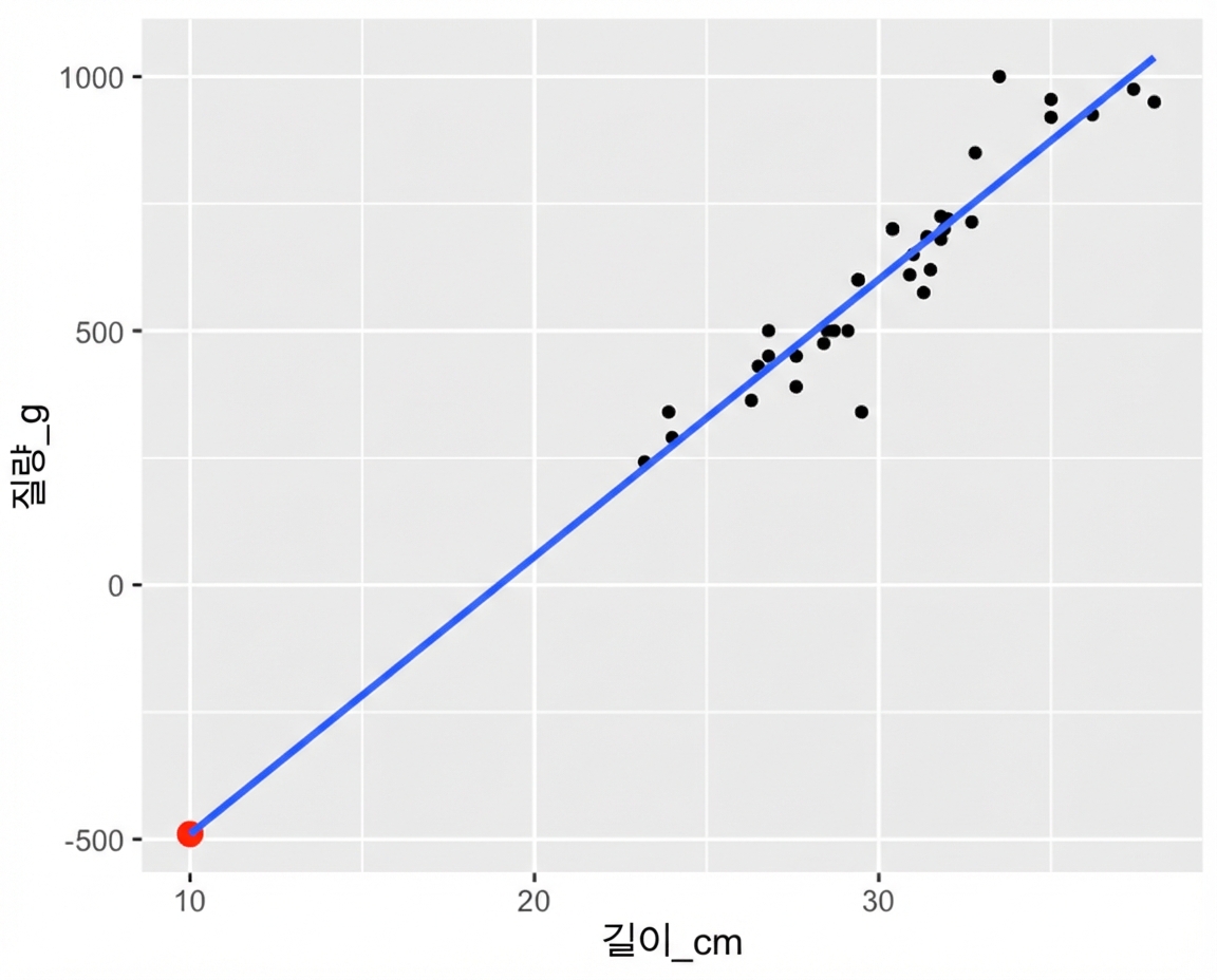
‘외삽’은 관측 범위 밖에서 예측하는 것을 의미합니다.

explanatory_little_bream <- tibble(length_cm = 10)
explanatory_little_bream %>% 
  mutate(
    mass_g = predict(
      mdl_mass_vs_length, explanatory_little_bream
    )
  )

# A tibble: 1 x 2
  length_cm mass_g
      <dbl>  <dbl>
1        10  -490.

연습해 봅시다!

R로 시작하는 회귀 분석