변수 변환

Python에서 statsmodels로 살펴보는 회귀 소개

Maarten Van den Broeck

Content Developer at DataCamp

농어 데이터셋

perch = fish[fish["species"] == "Perch"]
print(perch.head())

   species  mass_g  length_cm
55   Perch     5.9        7.5
56   Perch    32.0       12.5
57   Perch    40.0       13.8
58   Perch    51.5       15.0
59   Perch    70.0       15.7

유럽 농어, _Perca fluviatilis_

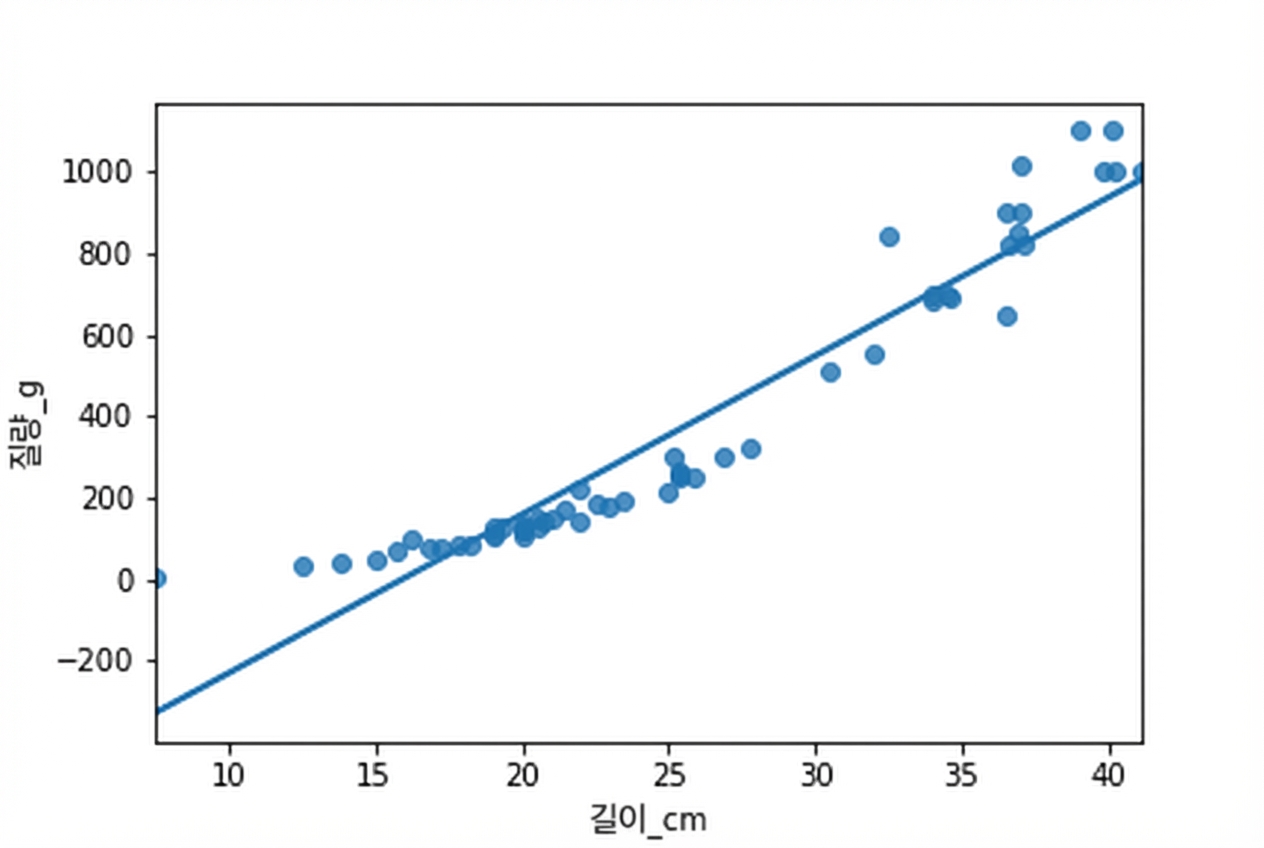
선형 관계가 아님

sns.regplot(x="length_cm",
            y="mass_g",
            data=perch,
            ci=None)

plt.show()

농어 무게 대 길이 산점도와 추세선. 농어는 길어질수록 선형보다 빠르게 무거워져 위쪽으로 굽은 곡선이 나타남.

잉어 대 농어

일반 잉어. 잉어는 몸이 납작함.

유럽 농어. 농어는 몸이 둥근 편임.

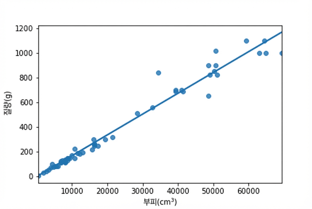
무게 대 길이의 세제곱 시각화

perch["length_cm_cubed"] = perch["length_cm"] ** 3

sns.regplot(x="length_cm_cubed",
            y="mass_g",
            data=perch,
            ci=None)
plt.show()

농어 무게 대 길이의 세제곱 산점도와 추세선. 변환 후 대부분의 점이 추세선 근처에 위치함.

무게 대 길이의 세제곱 모델링

perch["length_cm_cubed"] = perch["length_cm"] ** 3

mdl_perch = ols("mass_g ~ length_cm_cubed", data=perch).fit()
mdl_perch.params

Intercept         -0.117478
length_cm_cubed    0.016796
dtype: float64

무게 대 길이의 세제곱 예측

explanatory_data = pd.DataFrame({"length_cm_cubed": np.arange(10, 41, 5) ** 3,
                                 "length_cm": np.arange(10, 41, 5)})

prediction_data = explanatory_data.assign(
  mass_g=mdl_perch.predict(explanatory_data))
print(prediction_data)

   length_cm_cubed  length_cm       mass_g
0             1000         10    16.678135
1             3375         15    56.567717
2             8000         20   134.247429
3            15625         25   262.313982
4            27000         30   453.364084
5            42875         35   719.994447
6            64000         40  1074.801781

무게 대 길이의 세제곱 시각화

fig = plt.figure()
sns.regplot(x="length_cm_cubed", y="mass_g",
            data=perch, ci=None)
sns.scatterplot(data=prediction_data,
                x="length_cm_cubed", y="mass_g",
                color="red", marker="s")

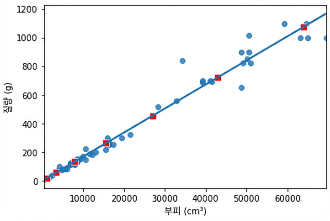
농어 무게 대 길이의 세제곱 산점도와 추세선. predict() 함수로 계산된 점이 표시되어 있으며, 점들이 추세선과 정확히 일치함.

fig = plt.figure()
sns.regplot(x="length_cm", y="mass_g",
            data=perch, ci=None)
sns.scatterplot(data=prediction_data,
                x="length_cm", y="mass_g",
                color="red", marker="s")

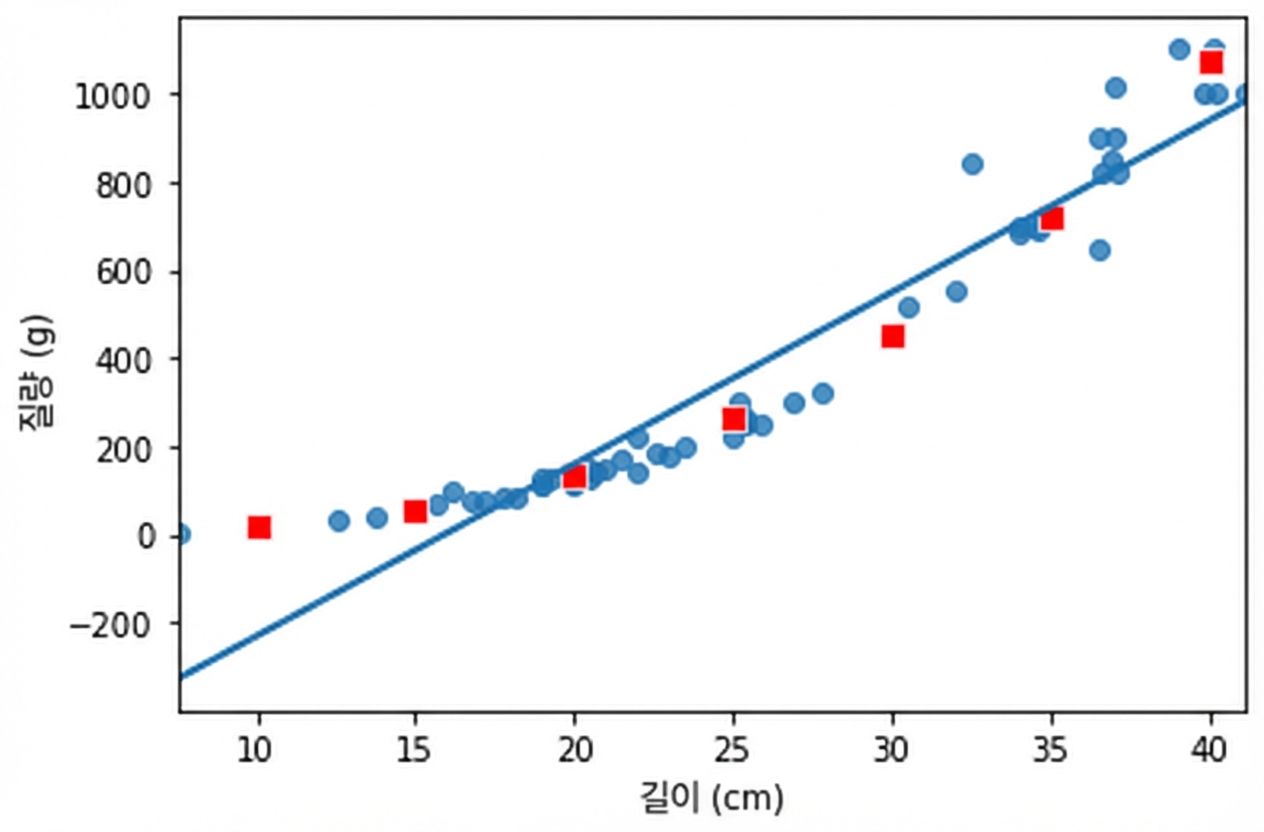
농어 무게 대 길이 산점도와 추세선. predict() 함수로 계산된 점이 추세선과 일치하지 않지만 데이터 점들의 곡선을 따름.

Facebook 광고 데이터셋

광고의 작동 방식

Facebook에 광고비를 지불합니다.
사람들이 광고를 봅니다("노출").
광고를 본 일부 사람들이 클릭합니다.

936개 행
각 행은 광고 1개를 나타냄

spent_usd	n_impressions	n_clicks
1.43	7350	1
1.82	17861	2
1.25	4259	1
1.29	4133	1
4.77	15615	3
...	...	...

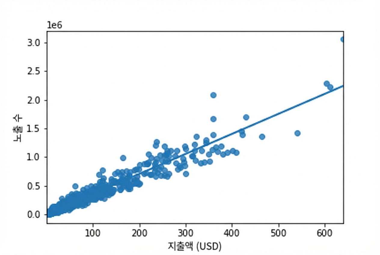
그래프가 밀집되어 있음

sns.regplot(x="spent_usd",
            y="n_impressions",
            data=ad_conversion,
            ci=None)

광고비 대 노출 수 산점도와 추세선. 대부분의 데이터 점이 그래프 왼쪽 하단에 밀집되어 있음.

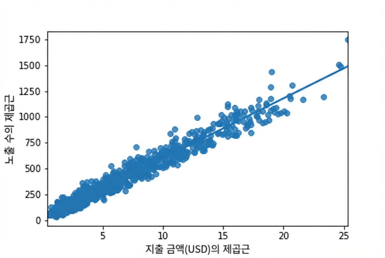
제곱근 대 제곱근

ad_conversion["sqrt_spent_usd"] = np.sqrt(
  ad_conversion["spent_usd"])

ad_conversion["sqrt_n_impressions"] = np.sqrt(
  ad_conversion["n_impressions"])

sns.regplot(x="sqrt_spent_usd",
            y="sqrt_n_impressions",
            data=ad_conversion,
            ci=None)

노출 수의 제곱근 대 광고비의 제곱근 산점도와 추세선. 이제 점들이 그래프 전체에 고르게 분포되어 있음.

모델링 및 예측

mdl_ad = ols("sqrt_n_impressions ~ sqrt_spent_usd", data=ad_conversion).fit()

explanatory_data = pd.DataFrame({"sqrt_spent_usd": np.sqrt(np.arange(0, 601, 100)),
                                 "spent_usd": np.arange(0, 601, 100)})

prediction_data = explanatory_data.assign(sqrt_n_impressions=mdl_ad.predict(explanatory_data),
                          n_impressions=mdl_ad.predict(explanatory_data) ** 2)
print(prediction_data)

   sqrt_spent_usd  spent_usd  sqrt_n_impressions  n_impressions
0        0.000000          0           15.319713   2.346936e+02
1       10.000000        100          597.736582   3.572890e+05
2       14.142136        200          838.981547   7.038900e+05
3       17.320508        300         1024.095320   1.048771e+06
4       20.000000        400         1180.153450   1.392762e+06
5       22.360680        500         1317.643422   1.736184e+06
6       24.494897        600         1441.943858   2.079202e+06

연습해 봅시다!

Python에서 statsmodels로 살펴보는 회귀 소개