Biểu đồ phân tán

Nhập môn trực quan hóa dữ liệu với ggplot2

Rick Scavetta

Founder, Scavetta Academy

48 geometries

geom_*
abline	contour	dotplot	jitter	pointrange	ribbon	spoke
area	count	errorbar	label	polygon	rug	step
bar	crossbar	errorbarh	line	qq	segment	text
bin2d	curve	freqpoly	linerange	qq_line	sf	tile
blank	density	hex	map	quantile	sf_label	violin
boxplot	density2d	histogram	path	raster	sf_text	vline
col	density_2d	hline	point	rect	smooth

Các loại biểu đồ phổ biến

Loại biểu đồ	Geom khả dụng
Phân tán	points, jitter, abline, smooth, count

Biểu đồ phân tán

Mỗi geom nhận các ánh xạ thẩm mỹ riêng, ví dụ geom_point():

Bắt buộc
x,y

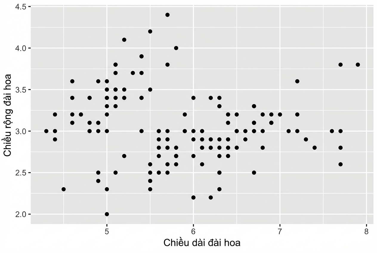
ggplot(iris, aes(x = Sepal.Length, 
                 y = Sepal.Width)) + 
  geom_point()

Biểu đồ phân tán

Mỗi geom nhận các ánh xạ thẩm mỹ riêng, ví dụ geom_point():

Bắt buộc	Tùy chọn
x,y	alpha, color, fill, shape, size, stroke

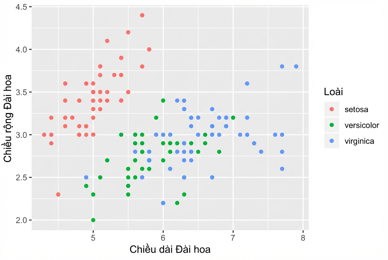
ggplot(iris, aes(x = Sepal.Length, 
                 y = Sepal.Width,
                 col = Species)) + 
  geom_point()

Ánh xạ thẩm mỹ theo geom

# Cả hai cho ra cùng một biểu đồ!
ggplot(iris, aes(x = Sepal.Length, y = Sepal.Width, col = Species)) + 
  geom_point()

ggplot(iris, aes(x = Sepal.Length, y = Sepal.Width)) + 
  geom_point(aes(col = Species))

Kiểm soát ánh xạ thẩm mỹ của từng layer độc lập:

head(iris, 3) # Dữ liệu thô

Species Sepal.Length Sepal.Width Petal.Length Petal.Width
1  setosa          5.1         3.5          1.4         0.2
2  setosa          4.9         3.0          1.4         0.2
3  setosa          4.7         3.2          1.3         0.2

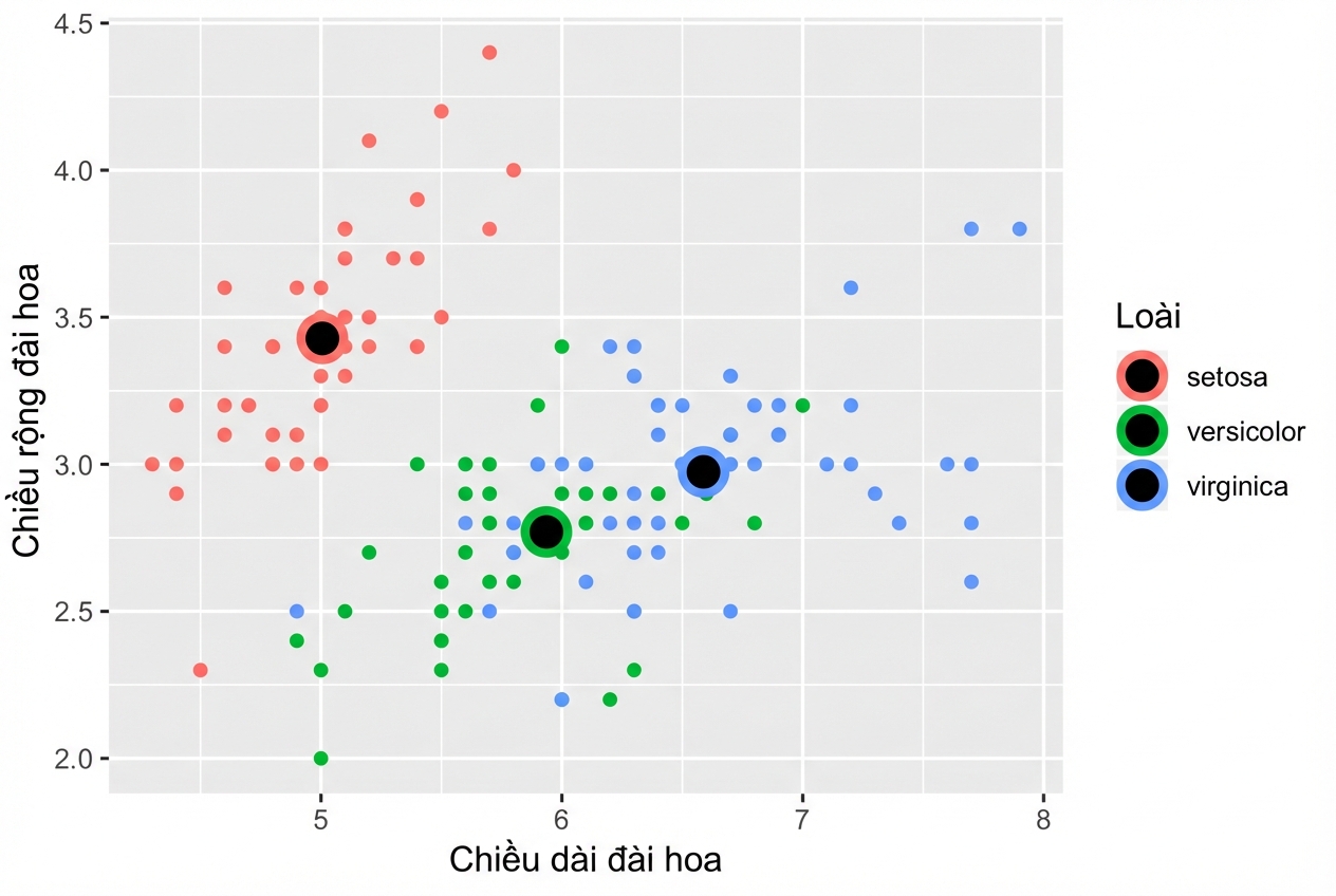
iris %>%
  group_by(Species) %>% 
  summarise_all(mean) -> iris.summary

iris.summary # Thống kê tóm tắt

# A tibble: 3 x 5
  Species    Sepal.Length Sepal.Width Petal.Length Petal.Width
  <fct>             <dbl>       <dbl>        <dbl>       <dbl>
1 setosa             5.01        3.43         1.46       0.246
2 versicolor         5.94        2.77         4.26       1.33 
3 virginica          6.59        2.97         5.55       2.03

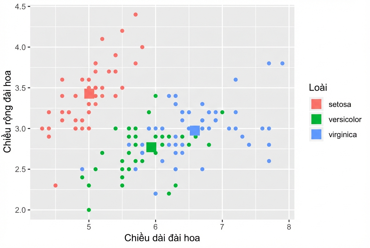
ggplot(iris, aes(x = Sepal.Length, y = Sepal.Width, col = Species)) +
  # Kế thừa cả dữ liệu và aes từ ggplot() 
  geom_point() + 
  # Dữ liệu khác, nhưng vẫn kế thừa aes
  geom_point(data = iris.summary, shape = 15, size = 5)

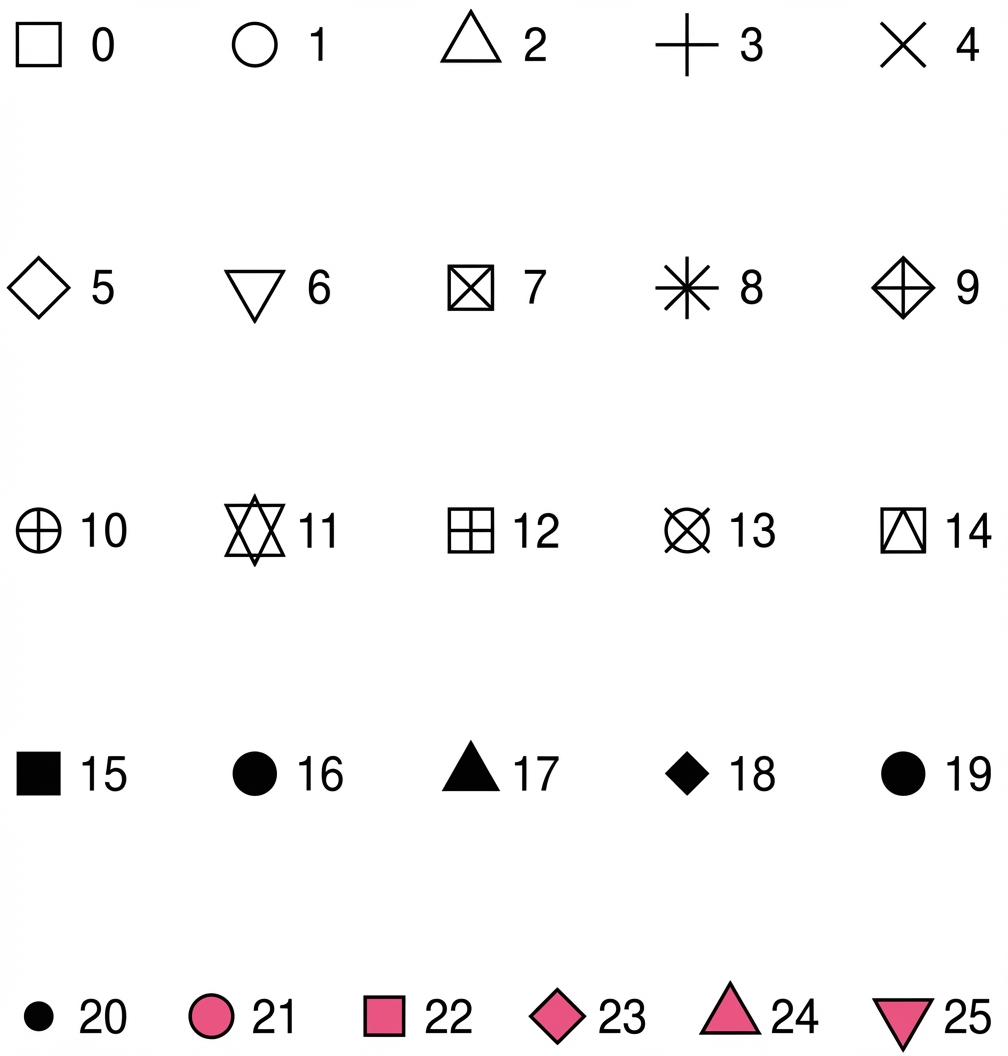
Giá trị thuộc tính shape

Ví dụ

ggplot(iris, aes(x = Sepal.Length, y = Sepal.Width, col = Species)) + 
  geom_point() +
  geom_point(data = iris.summary, shape = 21, size = 5, 
             fill = "black", stroke = 2)

Tính toán stats tức thời trong ggplot2

Xem khóa 2 để biết lớp stats.
Lưu ý: Tránh chỉ vẽ giá trị trung bình mà không có độ phân tán, ví dụ độ lệch chuẩn.

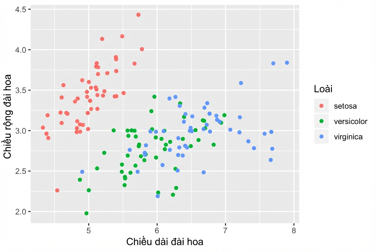
position = "jitter"

ggplot(iris, aes(x = Sepal.Length, y = Sepal.Width, col = Species)) + 
  geom_point(position = "jitter")

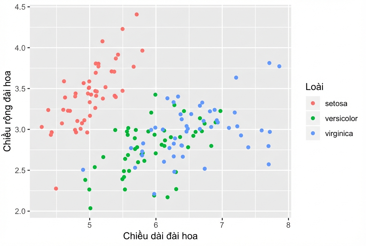
geom_jitter()

Lối tắt cho geom_point(position = "jitter")

ggplot(iris, aes(x = Sepal.Length, y = Sepal.Width, col = Species)) + 
  geom_jitter()

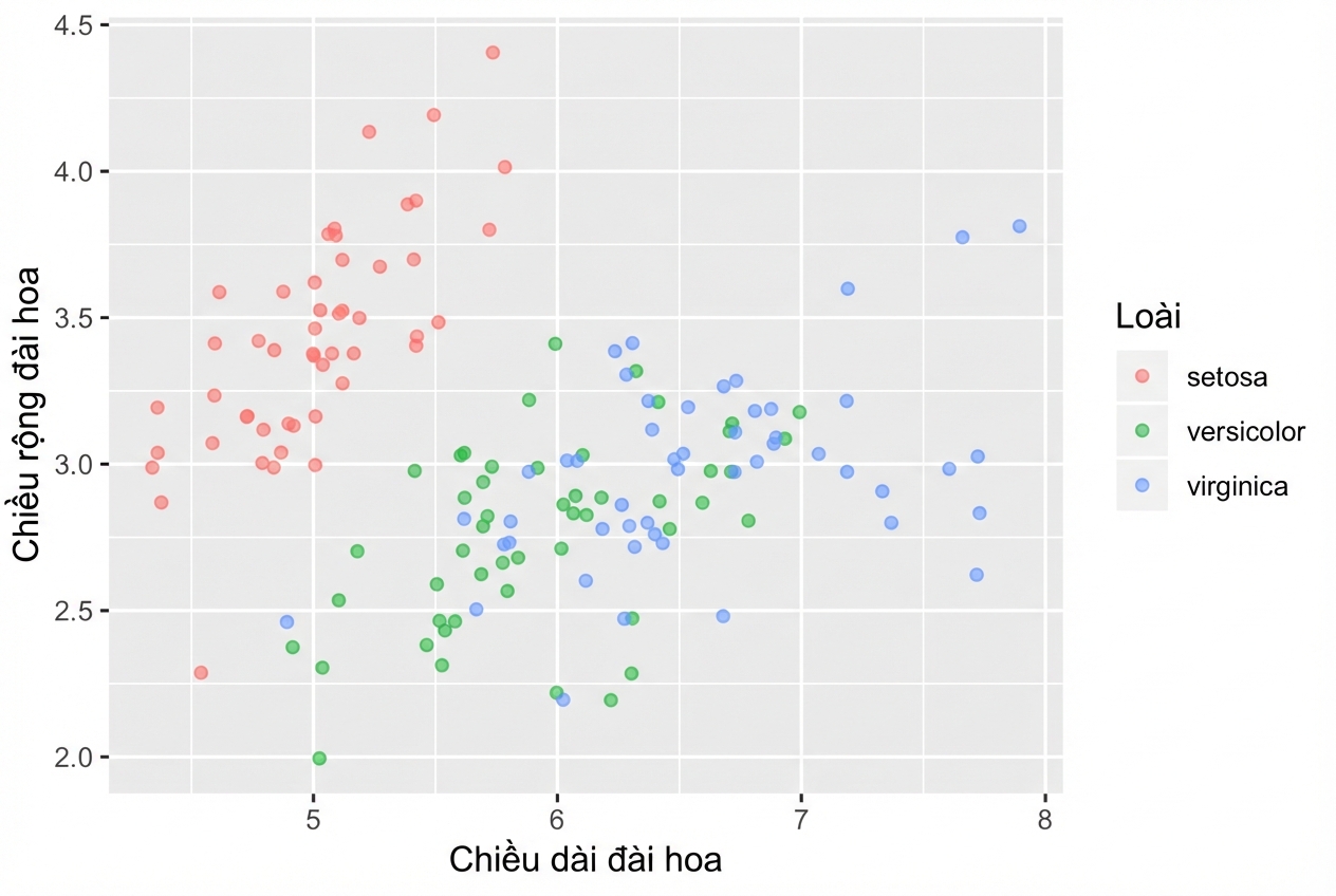
Đừng quên chỉnh alpha

Kết hợp jitter với alpha-blending khi cần

ggplot(iris, aes(x = Sepal.Length, y = Sepal.Width, col = Species)) + 
  geom_jitter(alpha = 0.6)

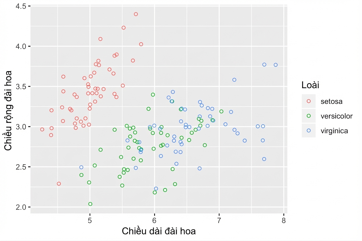
Vòng tròn rỗng cũng hữu ích

shape = 1 là vòng tròn rỗng.
Không cần dùng thêm alpha-blending.

ggplot(iris, aes(x = Sepal.Length, y = Sepal.Width, col = Species)) + 
  geom_jitter(shape = 1)

Ayo berlatih!

Nhập môn trực quan hóa dữ liệu với ggplot2