数値の説明変数が2つ

Rで学ぶ中級回帰分析

Richie Cotton

Data Evangelist at DataCamp

数値変数3個の可視化

3D散布図
応答を色で示す2D散布図

fishデータに列を追加

species	mass_g	length_cm	height_cm
Bream	1000	33.5	18.96
Bream	925	36.2	18.75
Roach	290	24.0	8.88
Roach	390	29.5	9.48
Perch	1100	39.0	12.80
Perch	1000	40.2	12.60
Pike	1250	52.0	10.69
Pike	1650	59.0	10.81

3D散布図

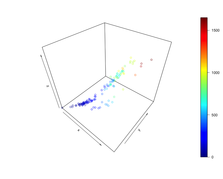
library(plot3D)

scatter3D(fish$length_cm, fish$height_cm, fish$mass_g)

library(plot3D)
library(magrittr)

fish %$%
  scatter3D(length_cm, height_cm, mass_g)

3D散布図

library(plot3D)
library(magrittr)

fish %$%
  scatter3D(length_cm, height_cm, mass_g)

3D散布図：魚の長さ×高さ×質量

2D散布図：色で応答を表現

ggplot(
  fish, 
  aes(length_cm, height_cm, color = mass_g)
) +
  geom_point()

散布図：色で応答（魚の長さ×高さ×質量）

Viridisカラースケール

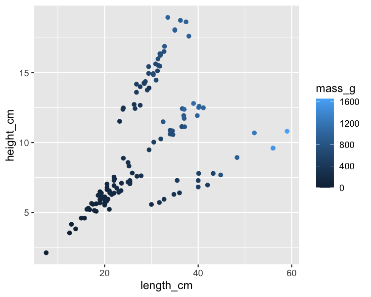
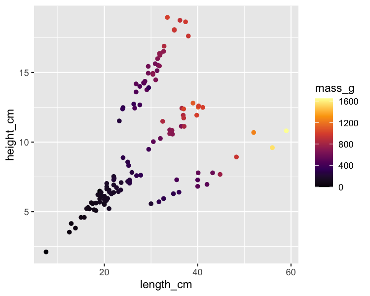
ggplot(
  fish, 
  aes(length_cm, height_cm, color = mass_g)
) +
  geom_point() +
  scale_color_viridis_c(option = "inferno")

散布図：Viridis（inferno）で色付け

数値の説明変数2つでモデリング

mdl_mass_vs_both <- lm(mass_g ~ length_cm + height_cm, data = fish)

Call:
lm(formula = mass_g ~ length_cm + height_cm, data = fish)

Coefficients:
(Intercept)    length_cm    height_cm  
    -622.16        28.97        26.34

予測の流れ

explanatory_data <- expand_grid(
  length_cm = seq(5, 60, 5),
  height_cm = seq(2, 20, 2)
)

prediction_data <- explanatory_data %>% 
  mutate(
    mass_g = predict(mdl_mass_vs_both, explanatory_data)
  )

予測のプロット

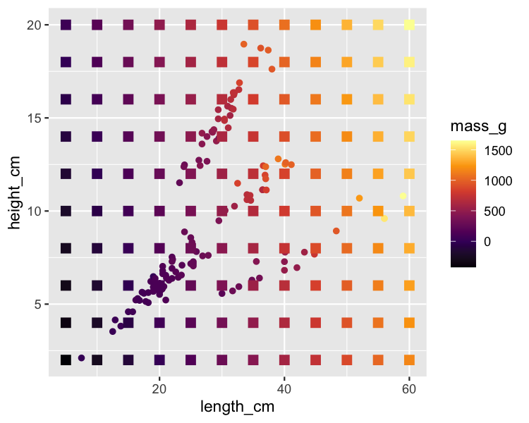
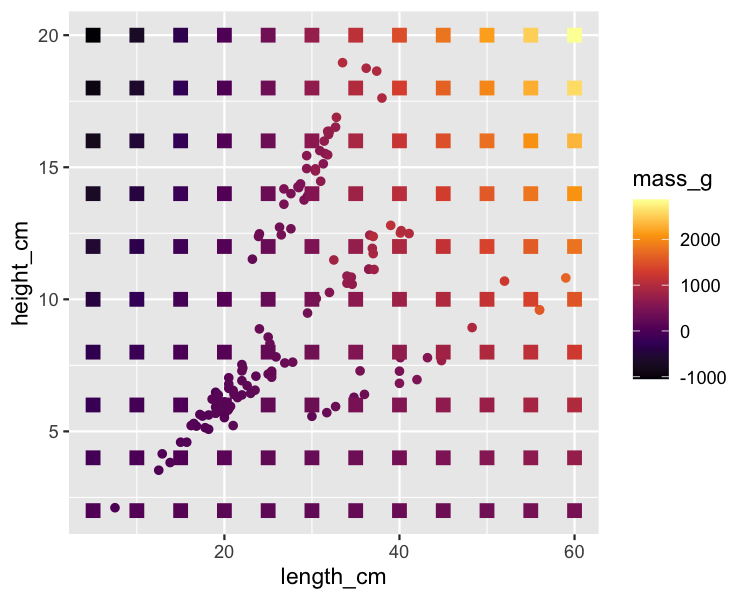
ggplot(
  fish, 
  aes(length_cm, height_cm, color = mass_g)
) +
  geom_point() +
  scale_color_viridis_c(option = "inferno") +
  geom_point(
    data = prediction_data, shape = 15, size = 3
  )

予測点を重ねた散布図（inferno）

交互作用の追加

mdl_mass_vs_both_inter <- lm(mass_g ~ length_cm * height_cm, data = fish)

Call:
lm(formula = mass_g ~ length_cm * height_cm, data = fish)

Coefficients:
        (Intercept)            length_cm            height_cm  length_cm:height_cm  
           159.1144               0.3001             -78.1234               3.5455

予測の流れ（再）

explanatory_data <- expand_grid(
  length_cm = seq(5, 60, 5),
  height_cm = seq(2, 20, 2)
)

prediction_data <- explanatory_data %>% 
  mutate(
    mass_g = predict(mdl_mass_vs_both_inter, explanatory_data)
  )

予測のプロット

ggplot(
  fish, 
  aes(length_cm, height_cm, color = mass_g)
) +
  geom_point() +
  scale_color_viridis_c(option = "inferno") +
  geom_point(
    data = prediction_data, shape = 15, size = 3
  )

予測点を重ねた散布図（交互作用あり）

練習しましょう！

Rで学ぶ中級回帰分析