モデルの説明

Pythonで学ぶ時系列解析

Rob Reider

Adjunct Professor, NYU-Courant Consultant, Quantopian

MA(1) モデルの数式表現

$\large \quad \quad \quad \quad R_t \ = \ \ \mu \ \ + \ \ \epsilon_t \ + \ \ \theta \ \epsilon_{t-1} $

右辺にラグ誤差が1つのみのため、以下と呼ばれます：
- 次数1の MAモデル、または
- MA(1) モデル
MAパラメータは $\large \theta$
$\theta$ のすべての値に対して定常

MA(1) パラメータの解釈

$\large \quad \quad \quad \quad R_t \ \ = \ \ \mu \ \ + \ \ \epsilon_t\ + \ \ \theta \ \epsilon_{t-1} $

$\large \theta$ が負：1期間の平均回帰
$\large \theta$ が正：1期間のモメンタム
注：1期間の自己相関は $\large \theta/(1+\theta^2)$（$\large \theta$ ではない）

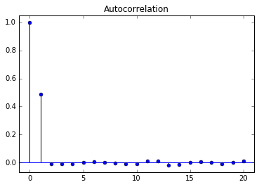
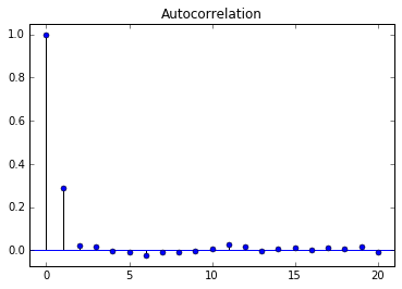
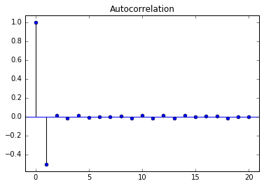
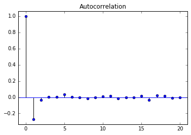
MA(1) 自己相関関数の比較

$\large \theta=0.9$
$\large \theta=0.5$

$\large \theta=-0.9$
$\large \theta=-0.5$

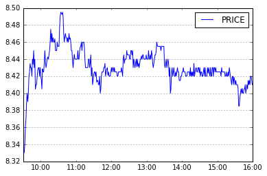
MA(1) プロセスの例：日中株式リターン

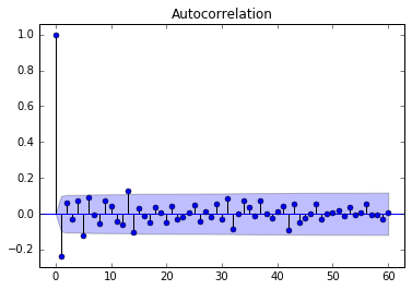
日中株式リターンの自己相関関数

高次MAモデル

MA(1)

$\large \quad \quad R_t = \mu + \epsilon_t - \theta_1 \ \epsilon_{t-1}$

MA(2)

$\large \quad \quad R_t = \mu + \epsilon_t - \theta_1 \ \epsilon_{t-1} - \theta_2 \ \epsilon_{t-2}$

MA(3)

$\large \quad \quad R_t = \mu + \epsilon_t - \theta_1 \ \epsilon_{t-1} - \theta_2 \ \epsilon_{t-2} - \theta_3 \ \epsilon_{t-3}$

...

MAプロセスのシミュレーション

from statsmodels.tsa.arima_process import ArmaProcess
ar = np.array([1])
ma = np.array([1, 0.5])
AR_object = ArmaProcess(ar, ma)
simulated_data = AR_object.generate_sample(nsample=1000)
plt.plot(simulated_data)

練習しましょう！

Pythonで学ぶ時系列解析

Preparing Video For Download...