利便抽出法

Rで学ぶサンプリング

Richie Cotton

Data Evangelist at DataCamp

Literary Digestの選挙予測
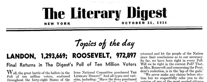
1936年のLiterary Digest紙の一面。選挙予測の見出し。ランドンは130万票、ルーズベルトは100万票弱と予測。

  • 予測:ランドン57%、ルーズベルト43%
  • 実際:ランドン38%、ルーズベルト62%
  • 標本が母集団を代表せず、標本バイアスが発生。
  • 最も手軽な方法で集めるのが利便抽出法。
Rで学ぶサンプリング

フランス人の平均年齢を求める

ディズニーランド・パリの写真。

  • ディズニーランド・パリで10人に調査。
  • 平均年齢は24.6歳。
  • これはフランス全体の良い推定になりますか?
1 Image by Sean MacEntee
Rで学ぶサンプリング

調査の精度は?

フランスの平均年齢
1975 31.6
1985 33.6
1995 36.2
2005 38.9
2015 41.2
  • 24.6歳は不適切な推定です。
  • ディズニー来園者は母集団を代表しません。
Rで学ぶサンプリング

利便抽出のコーヒー評価

coffee_ratings %>% 
  summarize(mean_cup_points = mean(total_cup_points))
  mean_cup_points
1           82.09
coffee_ratings_first10 <- coffee_ratings %>% 
  slice_head(n = 10)
coffee_ratings_first10 %>% 
  summarize(mean_cup_points = mean(total_cup_points))
  mean_cup_points
1            89.1
Rで学ぶサンプリング

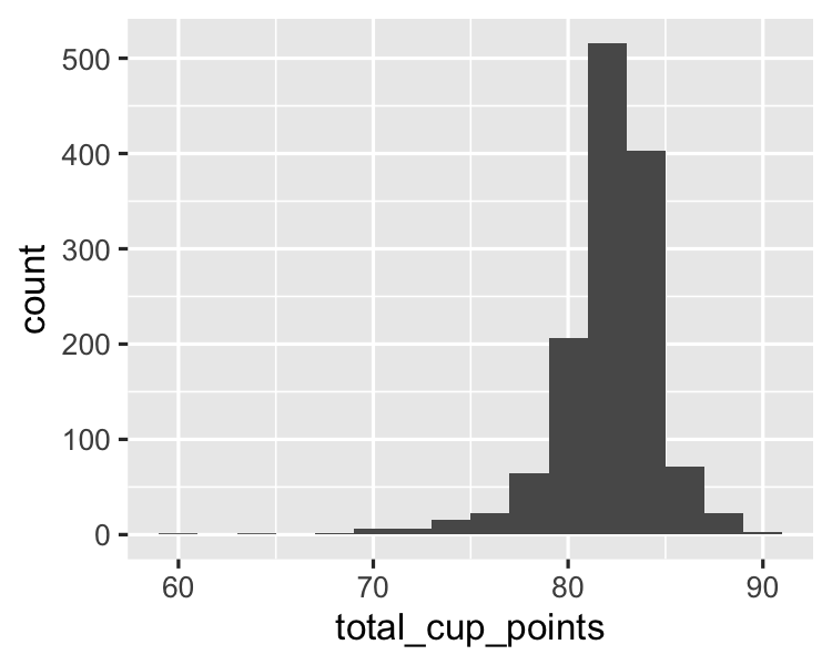
選択バイアスの可視化

coffee_ratings %>%
  ggplot(aes(x = total_cup_points)) +
  geom_histogram(binwidth = 2)

母集団のカップポイントのヒストグラム。

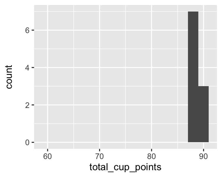
coffee_ratings_first10 %>%
  ggplot(aes(x = total_cup_points)) +
  geom_histogram(binwidth = 2) +
  xlim(59, 91)

サンプルのカップポイントのヒストグラム。

Rで学ぶサンプリング

選択バイアスの可視化 2

coffee_ratings %>%
  ggplot(aes(x = total_cup_points)) +
  geom_histogram(binwidth = 2) 

母集団のカップポイントのヒストグラム。

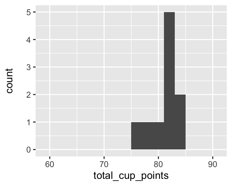
coffee_ratings %>%
  slice_sample(n = 10) %>% 
  ggplot(aes(x = total_cup_points)) +
  geom_histogram(binwidth = 2) +
  xlim(59, 91)

無作為抽出サンプルのカップポイントのヒストグラム。

Rで学ぶサンプリング

練習しましょう!

Rで学ぶサンプリング

Preparing Video For Download...