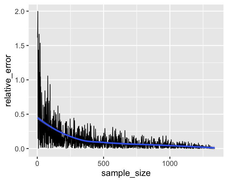
点推定の相対誤差

Rで学ぶサンプリング

Richie Cotton

Data Evangelist at DataCamp

サンプルは行数

coffee_ratings %>% 
  slice_sample(n = 300) %>% 
  nrow()

coffee_ratings %>% 
  slice_sample(prop = 0.25) %>% 
  nrow()

coffee_ratings %>% 
  summarize(mean_points = mean(total_cup_points)) %>% 
  pull(mean_points)

82.15

coffee_ratings %>% 
  slice_sample(n = 10) %>% 
  summarize(mean_points = mean(total_cup_points)) %>% 
  pull(mean_points)

82.82

coffee_ratings %>% 
  slice_sample(n = 100) %>% 
  summarize(mean_points = mean(total_cup_points)) %>% 
  pull(mean_points)

82.02

coffee_ratings %>% 
  slice_sample(n = 1000) %>% 
  summarize(mean_points = mean(total_cup_points)) %>% 
  pull(mean_points)

82.16

母数

population_mean <- coffee_ratings %>% 
  summarize(mean_points = mean(total_cup_points)) %>% 
  pull(mean_points)

点推定

sample_mean <- coffee_ratings %>% 
  slice_sample(n = sample_size) %>% 
  summarize(mean_points = mean(total_cup_points)) %>% 
  pull(mean_points)

相対誤差（％）

100 * abs(population_mean - sample_mean) / population_mean

ggplot(errors, aes(sample_size, relative_error)) +
  geom_line() +
  geom_smooth(method = "loess")

相対誤差とサンプルサイズの散布図。

Rで学ぶサンプリング